Integrated Applications
Volt-var Optimization (VVO)
The sample VVO application is a Python implementation of a heuristic method that PNNL has investigated before [CIT3], [CIT4], [CIT5]. There are more advanced VVO methods that will be implemented in future work.
Visualization
We have created a web-based visualization of the sample VVO application. The visualization displays the topology of the IEEE 8500-Node system as an interactive graph. Capacitors and regulators are highlighted in the graph and displayed alongside tables with current values for capacitor status (OPEN or CLOSED), regulator voltage, and feeder power.
State Estimator Service
Given a perfect and complete set of voltage magnitude and angle measurements, along with a detailed and accurate power system model, one could calculate the real power, or any other electrical variable of interest, anywhere in the system. In practice, measurements have errors, time delays, and may even be missing. State estimation refers to the process of minimizing the errors and filling in gaps [1]. One state estimation method is called “weighted least squares”, and it’s analogous to drawing the best-fit line through a set of scattered points. Other methods may perform better [2]. Also, on distribution systems, it may be better to estimate branch currents instead of node voltages, but the principle is the same. In GridAPPS-D, the visualizations and applications ought to use the best available state estimator outputs, instead of raw SCADA values, for both accuracy and consistency. Therefore, the state estimator is not an application but a service in GridAPPS-D, sitting between emulated SCADA and the GOSS bus.
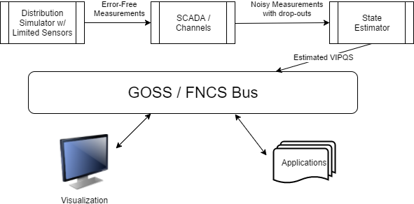
Figure 1: The state estimator processes noisy and incomplete measurements, then posting estimated voltage (V), current (I), real power (P), reactive power (Q) and switch status (S) values onto the GridAPPS-D message / data bus.
In Figure 1, the power system model (upper left) will include a limited number of sensors, corresponding to actual voltage and current transformers, line post sensors, wireless sensors, etc. In some scenarios, smart meters can also be sensors. Each such sensor will have different performance characteristics (e.g. precision, accuracy, sampling rate). Distribution systems typically do not have enough sensors to make the system observable, so there will be measurement gaps in the topology. The state estimator might fill these gaps with interpolation and graph-tracing methods on the power system model.
The supervisory control and data acquisition (SCADA) system in Figure 1 introduces more errors and failure points. Eventually, GridAPPS-D may simulate these impacts by federating ns-3 as a co-simulator. Until then, a placeholder module could be used to insert variable errors, time delays and dropouts in each measurement, whether due to sensor characteristics or the communication system. The output represents data as it would come into an operations center, and feeds the state estimator. Internally, the data flows between simulator, SCADA and state estimator might be implemented with FNCS, but this is an implementation detail. The state estimator will provide two outputs to the GOSS bus used by all GridAPPS-D applications:
- At a time step configured by the platform, publish the best-estimate VIPQS values wherever sensors actually exist in the model, with quality attributes that still have to be established. Sensor locations delineate circuit segments, and note that all VIPQS values will be estimated at the boundaries, even if the sensor measures only V or I, for example.
- Upon request by another application or service, publish the estimated VIPQS values for all nodes and components in the model, even at locations where no sensors exist. A variant is to publish the estimates only for selected nodes and components.
As indicated in Figure 1, other applications need to obtain estimated VIPQS values from the GOSS bus. Switch open/close states are a special case; they might be considered known values, but in practice the switch state is a measurement, which could lead to topology errors in the model. For GridAPPS-D, switch state estimates need to be a point of emphasis. Given that most distribution systems lack redundant measurements, It would be possible for an application to query these VIPQS values directly from the simulator or SCADA, bypassing the state estimator, but this is “cheating” in most situations. However, in the application development process, idealized VIPQS values could be obtained through a combination of two methods:
- Add more sensors to the power system model
- Set the sensor and channel errors to zero
Because the sensor outputs in GridAPPS-D come from a power flow solution that enforces Kirchhoff’s Laws, the state estimator will produce ideally accurate values whenever the sensor and channel errors have been specified to be zero. The state estimator may still exhibit interpolation errors between sensor locations, but that is readily mitigated for testing purposes by adding more sensors.
With reference to RC1, the visualization and VVO applications should now subscribe to VIPQS values from the state estimator, not from the distribution simulator. They may also use or display quality metrics on the estimated values.
Design Objectives
State estimation is widely used in transmission system operations but is less common in distribution system operations due to a relatively limited value in traditional distribution systems, additional computational complexity, and a lack of sensors. Advanced distribution management platforms like GridAPPS-D provide access to model and sensor data that can be leveraged to overcome barriers to adoption and open the door to distribution system state estimators that are fast and accurate enough to be useful in utility operations.
A distribution system state estimator computes the most likely state given a set of present and/or past measurements. The full state of a distribution system consists of either the full set of complex bus voltages or the full set of complex branch currents; given the system model (admittance matrix), the remaining system parameters can be computed given the full system state.
Use Cases
- Assist power factor optimization: Utility objective is unity power-factor at the substation.
- Assist voltage optimization (planning): Utility objective is 1 p.u. voltage at last house primary.
- Real-time state estimation for advanced applications: applications can access the state estimate at a sufficient resolution to capture e.g. insolation variation caused by clouds.
Algorithms
State estimation uses system model information to produce an estimate of the state vector x given a measurement vector z. The measurement vector is related to the state vector and an error vector by the measurement function, which may be non-linear.
Multiple formulations of the distribution system state estimation problem are possible:
- Node Voltage State Estimation (NVSE): The state vector consists of node voltage magnitudes and angles for each node in the system (one reference angle can be eliminated from the state vector). This formulation of the state estimation problem is general to any topology and it is the standard for transmission system state estimation.
- Branch Current State Estimation (BCSE): Radial topology and assumptions about shunt losses create a linear formulation of the state estimation problem. The state vector contains branch currents and, for a fully-constrained problem, requires one state per load, which can be less than the number of branches in the system.
Different algorithms provide different advantages for distribution system state estimation. A subset of the state estimation algorithms below will be used to achieve these goals.
- Weighted Least Squares Estimation (WLSE): a concurrent set of measurements are used to find a state vector that minimizes the weighted least squares objective function. The algorithm is memoryless with respect to previous solutions and measurements should be synchronized.
- Kalman Filter Estimation (KFE) and Extended Kalman Filter Estimation (EKFE): The Kalman filter provides a mechanism to consider past state estimates alongside present measurements. This provides additional noise rejection and allows asynchronous measurements can be considered individually. KFE is appropriate for linear BCSE and EKFE is compatible with nonlinear NVSE.
- Unscented Kalman Filter Estimation (UKFE): The unscented transform estimates the expected value and variance of the system state by observing the system outputs for inputs spanning the full dimensionality of the measurement space. Again, the Kalman filter provides a mechanism to consider past estimates.
TRL
The state estimator application will provide the capability to estimate the full system state using asynchronous measurement data. In addition a model order reduction technique will be implemented to greatly speed up the state estimation computation and to reduce the dependence on forecast-based pseudo-measurements. A paper (Reduced-Order State Estimation for Power Distribution Systems with Sparse Sensing) is targeted for IEEE Transactions on Power Systems.
Architecture
The state estimation service is being developed in c++. A modern c++ implementation allows the application to adapt to an evolving interface. The program architecture is shown below.
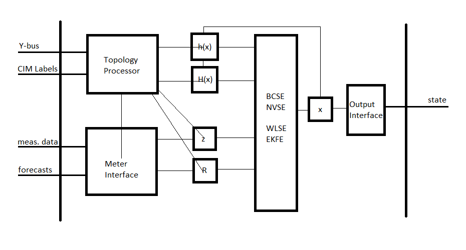
Topology Processor: initializes the measurement function and its Jacobian and determines the size of the measurement vector, the measurement covariance matrix, and the state vector.
Meter Interface: updates the measurement vector and the measurement covariance matrix as new measurement data comes available.
State Estimator: performs the state estimation operation according to the specified algorithm.
Output Interface: formats the state vector and any implicit states as an output stream.
Inputs
Upon initialization, the topology processor will receive the Y-bus from the GridLAB-D service and will query contextual information and sensor locations from the CIM database.
Periodic measurement data, including any forecasts to be used a pseudo-measurements will be required as inputs.
A “terminate” command from the platform will end the state estimation process.
Outputs
The output will include the full system state (node voltages and/or branch currents TBD).
Testing and Validation
Evaluation metrics
- State Error: compare state estimation output to “true” system state.
- Accuracy over baseline: compare state error of state estimator to state error of a QSTS load-flow model.
- Execution Time
- Bad Sensor Detection (binary)
Scenarios
- Full sensor deployment: verify that the true system state can be reproduced.
- Sparse sensor deployment: verify that the state estimator performs better than a QSTS load-flow model.
- Breaker trip: verify that switch state can be detected even when it is reported incorrectly.
- Bad sensor detection: verify that a sensor that is producing bad data can be identified.
- Dependent application support: verify that the state estimator can support e.g. the VVO application.
- Fault: for a radial system, determine the nearest common bus from multiple emulated customer calls.
Operating/Running
The state estimator will execute the topology processor at initialization and will enter a stat estimation loop. The state estimation loop will exit and the process will end upon receiving a ‘terminate’ command from the platform.
At initialization, a configuration file will be read for:
- State estimation mode (state vector and algorithm) selection
- Normalized residual threshold for bad measurement / sensor detection
References
[1] T. E. McDermott, “Grid Monitoring and State Estimation,” in Smart Grid Handbook, ed: John Wiley & Sons, Ltd, 2016.
[2] A. Abur and A. Gómez Expósito, Power system state estimation : theory and implementation. New York, NY: Marcel Dekker, 2004.
[3] M. E. Baran and A. W. Kelley, “A branch-current-based state estimation method for distribution systems,” in IEEE Transactions on Power Systems, vol. 10, no. 1, pp. 483-491, Feb 1995.
[4] Z. Jia, J. Chen and Y. Liao, “State estimation in distribution system considering effects of AMI data,” 2013 Proceedings of IEEE Southeastcon, Jacksonville, FL, 2013, pp. 1-6.
[5] S. C. Huang, C. N. Lu and Y. L. Lo, “Evaluation of AMI and SCADA Data Synergy for Distribution Feeder Modeling,” in IEEE Transactions on Smart Grid, vol. 6, no. 4, pp. 1639-1647, July 2015.
[6] M. Kettner; M. Paolone, “Sequential Discrete Kalman Filter for Real-Time State Estimation in Power Distribution Systems: Theory and Implementation,” in IEEE Transactions on Instrumentation and Measurement, vol.PP, no.99, pp. 1-13, Jun. 2017.
[7] G. Valverde and V. Terzija, “Unscented kalman filter for power system dynamic state estimation,” in IET Generation, Transmission & Distribution, vol. 5, no. 1, pp. 29-37, Jan.
Model Validation Application
The state estimator basically attempts to fit measured data to a power flow model, usually assuming that the model is correct. However, a model attribute (e.g. line impedance) could also be estimated by minimizing its error residual in the state estimator’s power flow solution. This process works best when applied to just one or a few suspect attributes, and/or when an archive is available to provide enough redundant measurements. The Model Validation Application will use these state estimator features off-line to help identify and correct the following types of model errors:
- Unknown or incorrect service transformer sizes
- Unknown or incorrect secondary circuit lengths
- Incorrect phase identification of single-phase components
- Phase wiring errors in line segments and switches
- Transformer connection errors, especially reversed primary and secondary
- Primary conductor sizes that don’t decrease monotonically with distance from the source
- Missing regulator and capacitor control settings (i.e. supply defaults from heuristic rules)
- More than one of these on the same pole: recloser, line regulator, capacitor
- Substation transformer impedance and turns ratio
These types of errors often appear upon the initial model import from a geographic information system (GIS), or in periodic model updates from GIS. Other error types may be added later. Many utilities do not have their secondary circuits modeled at all, but this has an important impact on AMI data. The service transformers and secondary circuits insert significant impedance between AMI meters and the primary circuit, where most of the other sensors are installed. Therefore, the first two items will require AMI data, and also enable its more effective use.
As shown in Figure 1, the Model Validator integrates with GridAPPS-D as a hosted application on the GOSS bus. Internally, it will use some of the same algorithms as the State Estimator and may share some code or binary files, but this is an implementation detail. It will need to access an archive of state-estimated VIPQS data, which may include AMI data. It will also use or incorporate an off-line power flow model, not the same one running in the GridAPPS-D distribution simulator. This may be EPRI’s OpenDSS simulator [1]; compared to GridLAB-D, it’s more tolerant of model errors and provides more diagnostic information about model errors.
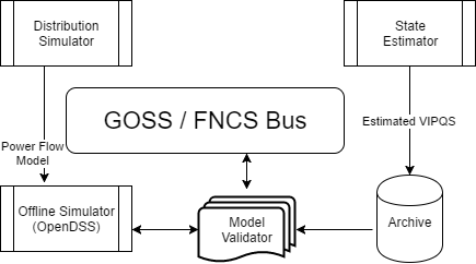
Figure 1: The Model Validator works with an archive from the state estimator, and an off-line power flow model.
Design Objectives
The model validator will detect and attempt to correct unreasonable component interconnections and network parameters. The model validation application will be implemented in Python.
Use Cases
- Valid transformer size and orientation (Utility): orientation is not captured explicitly in their GIS system.
- Discover secondary line impedance parameters (Utility) conductor type and line length are currently based on generic assumptions.
- Sanity check or estimate transformer size and impedance.
- Verify that the nominal voltage of nodes matches the base voltage of the segment: generally the winding voltage of the upstream transformer or swing bus voltage.
- Sanity check conductor sizes and line current ratings.
- Validate and fill in regulator and capacitor control settings.
- Check phase continuity (GridLAB-D may not model phase discontinuities)
Inputs
The model validator will have access to the CIM database and archived data from the state estimator.
Outputs
The model validator will one or both of the following outputs:
- Model status: log file or GUI pipe for identified issues.
- Model correction: CIM updates to correct identified issues.
Testing and Validation
Evaluation metrics
- Ability to detect known issues.
Scenarios
- Utility merger: models with different format may be interpreted differently, creating issues a CIM model.
- Data entry issue: model update does not match upgrade performed in the field
Operating/Running
The model validator script will execute once when called by the platform.
At initialization, a configuration file will be read for:
- Mode (status, quiet, verbose; see outputs section)
- Selectable validation items (use cases)
References
[1] R. C. Dugan and T. E. McDermott, “An open source platform for collaborating on smart grid research,” in Power and Energy Society General Meeting, 2011 IEEE, 2011, pp. 1-7.
Transactive Systems Application
Transactive energy is a method of controlling loads and resources on the distribution system, combining both market and electrical principles [1]. One reason for including this application in DOE-funded GridAPPS-D is that PNNL has made several technical contributions and led several demonstration projects in transactive systems, also funded by DOE [2].
Application structure
This transactive systems application is to be implemented as a modularized 2-layer 3-level structure, as seen from Figure 3. The layer decomposition helps the control of various groups, with limited information flow between different layers. With the predefined functions in each agent type (Agent A, B, and C) in each level, the existing transactive system related work can be conveniently integrated into the application, and the new control features can be added into specific control function in each type of the agent easily.
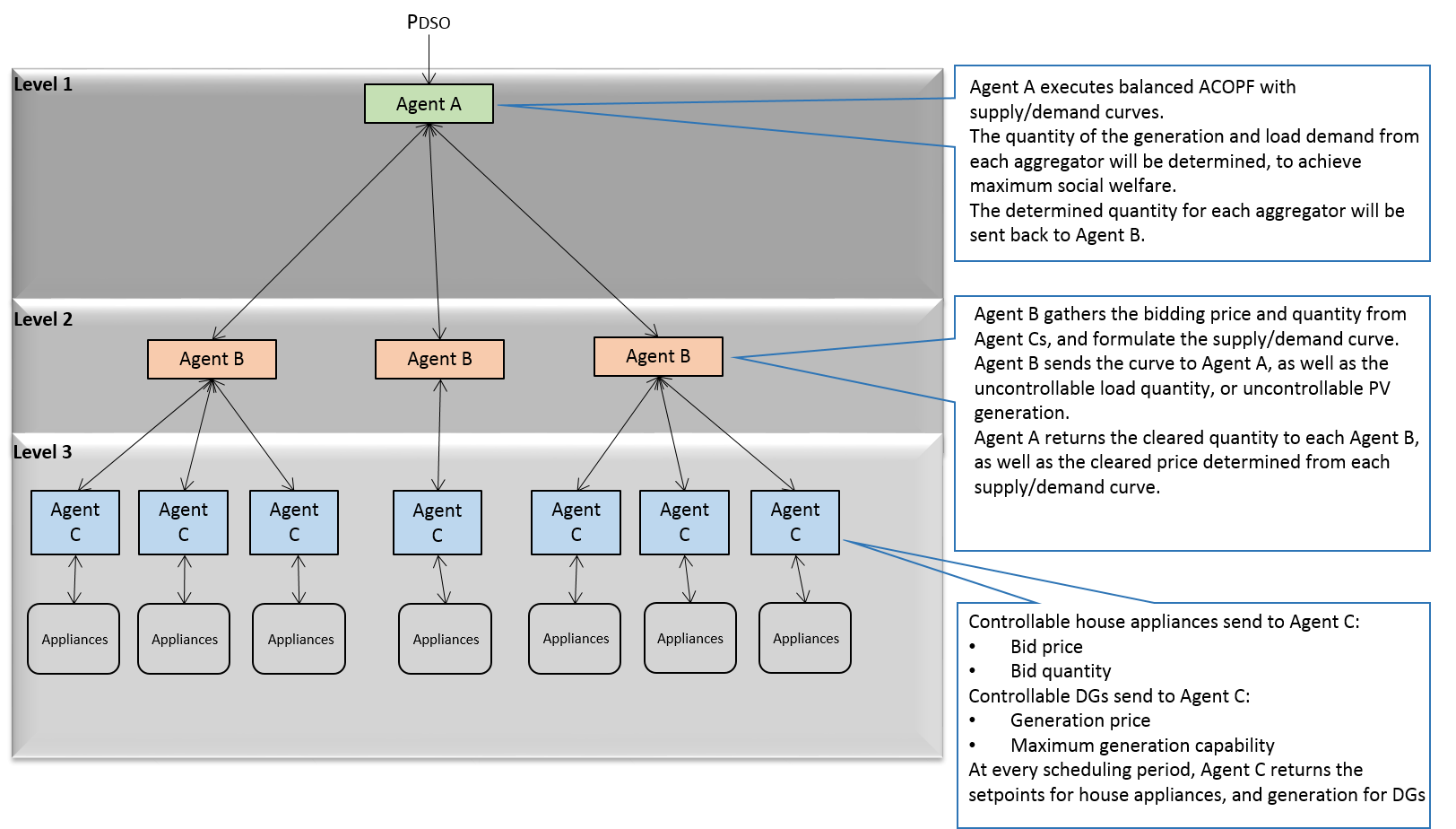
Figure 3: The structure of the modularized 2-layer 3-level transactive system application
The modularized agents opens the door for integrating different control mechanisms into the application. Users need to consider which level their control algorithm fits into, and fill in the control function of the Agent class in that level, without worrying about communications between the agents. In each level, the same type of the agent may have various control functions, which help combining benefits of different control schemes together.
Agent A, B and C will be implemented as VOLTTRON applications. VOLTTRON is an application platform for distributed sensing and control applications [3]. With the capability of hardware-in-the-loop (HIL) testing through VOLTTRON, the transactive systems application will be tested using the actual devices. A GOSS-VOLTTRON Bridge is to be implemented, for the communication between GridAPPS-D and the VOLTTRON agents in the transactive systems application.
Application test cases
The hierarchical control framework introduced in [4] for integrated coordination between distributed energy resources and demand response will be implemented into the application. In addition, [4] has not considered the power losses or power constrains, which will be taken into consideration in this test case. The two-layer control mechanism, including the coordination layer and device layer, fits the proposed structure of the application well. The control in each level will be implemented into corresponding function in each type of the agent. The IEEE 123-node test feeder built in GridLAB-D will be used for testing the application.
CIM extension for the Application
The latest versions of GridAPPS-D has used a reduced-order CIM to support feeder modeling. With transactive system application included into GridAPPS-D platform, more objects, such as house air conditioner and water heater, need to be defined in CIM. Before the definition in CIM, a simplified version of the house object and water heater object are to be implemented in GridLAB-D.
References
[1] Gridwise Architecture Council. (2017). Transactive Energy. Available: http://www.gridwiseac.org/about/transactive_energy.aspx
[2] Pacific Northwest National Laboratory. (2017). Transactive Energy Simulation Platform (TESP). Available: http://tesp.readthedocs.io/en/latest/
[3] S. Katipamula, J. Haack, G. Hernandez, B. Akyol, and J. Hagerman, “VOLTTRON: An Open-Source Software Platform of the Future,” IEEE Electrification Magazine, vol. 4, pp. 15-22, 2016.
[4] Di Wu, Jianming Lian, Yannan Sun, Tao Yang, Jacob Hansen, “Hierarchical control framework for integrated coordination between distributed energy resources and demand response,” Electric Power Systems Research, pp. 45-54, May 2017.
Distribution Optimal Power Flow for Real-Time Setpoint Dispatch
Objectives
This application is designed to address the problem of optimizing the operation of aggregations of heterogeneous energy resources connected to a distribution system. We will focus on real=time optimization method and the power setting points of the distributed energy resources (DERs) will be updated on a second or subsecond timescale to maximize the operational objectives while coping with the variability of ambient conditions and noncontrollable energy assets [1]. In order to avoid massive measurements and overcome the limitation caused by model inaccuracy, this application will be implemented in a distributed manner, and only local measurements and a feedback signal from the substation aggregator are needed to determine the optimal setpoints for each controlled DER unit.
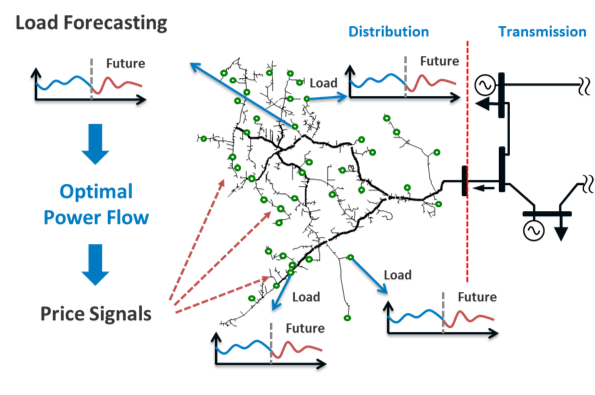
Figure 1 The conceptual framework of distribution OPF for real=time setpoint dispatch.
Figure 1 shows the conceptual framework of this application, and this application is targeting at TRL 3.
Design
Figure 2 describes the overall work flow of the application. Distribution OPF algorithm requires real=time measurements, distribution system model and power flow results, which will be obtained from GridAPPS=D platform through GOSS/FNCS message bus. The optimization problem formulation can be constructed using user=defined cost functions for different controllable devices. Finally the optimal setpoints for controllable devices will be solved based on the feedback information from system measurements. These setpoints will be sent back to GridLab=D grid model to update DER operations. Such a closed=loop control forms the control iteration for the studied time point, and new setpoints for the following time points will be determined in the same manner using the updated model and measurements.
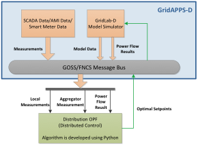
Figure 2 The workflow of real=time setpoint dispatch application and its interaction with GridApps=D.
Data requirements
The DER application requires p and q values from the inverters attached to PVs, loads, and capacitors. The DER application also requires setting the p and q values of inverters attached to PVs.
Testing and Validation
Evaluation metrics of this application:
- Real/reactive power at the substation
- System loss
- Voltages across the entire distribution grid: voltage magnitude, voltage fluctuation, voltage unbalance.
- Legacy control device operations: total control actions of all capacitors and regulators
Scenarios:
- Optimal Dispatch for Distributed PV Systems
- Optimal Dispatch for Distributed PV + Energy Storage
- Etc. (will be added when implementing the application)
Operating/Running
This application will be developed using Python.
References
[1] E. Dall’Anese, A. Bernstein, and A. Simonetto, “Feedback=based Projected=gradient Method for Real=time Optimization of Aggregations of Energy Resources,” IEEE Global Conference on Signal and Information Processing (GlobalSIP), Montreal, Canada, Nov. 2017.
Short-Term Grid Forecasting
Objectives
Today’s distribution systems have been experiencing a significant transformation due to an increasing amount of smart electric loads and distributed energy resources, such as electric vehicles, smart home appliances, rooftop photovoltaic systems, and energy storage. As more flexible resources integrated into distribution systems, coordination among various flexible resources plays an important role in distribution system operations to optimally manage distribution assets and flexible resources. On the other hand, with the increasing penetration of variable energy resources, it is crucial for system operators to not only monitor and estimate the current grid conditions but also forecast the future system status, which allows for proactive dispatch of controllable resources and better preparation for ever-changing grid conditions. This application develops predictive locational marginal prices (DLMPs) to proactively manage the distribution assets and flexible resources based on forecasted grid conditions. This application enables the distribution system operators to optimally incentivize individual resources to achieve system-level control objectives, such as minimizing total generation cost and optimizing the voltage profile; and it paves the way to a fully functional distribution market with granular prices that reflect the time- and location-specific values of individual participants.
Design
This application develops a high-resolution, short-term load forecasting method to accurately predict the power consumption of individual customers in distribution systems. Using historical load measurements as inputs, it trains a support vector regression model to forecast the future load. Based on the forecasted load in the short-term future, this application develops a three-phase AC optimal power flow problem to determine the predictive DLMPs in distribution systems. By accurately modeling the losses and the imbalances of distribution networks, it provides time- and location-specific pricing of individual resources.
Operating/Running
The application was built using Python 3.6. It will be run from the platform GUI.
References
[1] H. Jiang, Y. Zhang, E. Muljadi, J. J. Zhang, and D. W. Gao, “A Short-Term and High-Resolution Distribution System Load Forecasting Approach Using Support Vector Regression with Hybrid Parameters Optimization,” in IEEE Transactions on Smart Grid, vol. 9, no. 4, pp. 3341-3350, July 2018. [2] R. Yang and Y. Zhang, “Three-Phase AC Optimal Power Flow Based Distribution Locational Marginal Price,” IEEE Innovative Smart Grid Technologies, Arlington, VA, Apr. 2017.
Solar Forecasting Application
Objectives
When observations of solar radiation are limited, persistence and smart persistence solar forecasting techniques are frequently the easiest and most effective methods to use. Often though, these techniques suffer from having no information about current cloud properties, which could improve the forecast. At NREL, a Physics-based Smart Persistence model (PSPI) [1] was created for intra-hour solar forecasting using only GHI observations and a cloud retrieval technique. This model breaks down common solar radiation components such as GHI and solar zenith angle (SZA) using a two-stream approximation [2] and methods used in [3] to forecast future GHI, cloud fraction, and cloud albedo. With this information, this technique can then be used to forecast solar power (still in development). Figure 1 below shows the conceptual framework for PSPI.
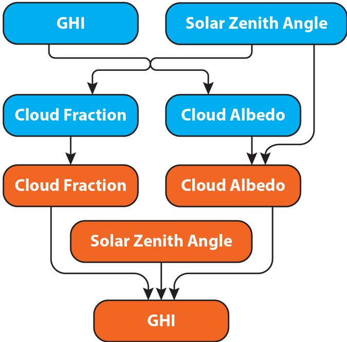 Figure 1 Conceptual framework for PSPI. PSPI breaks up the GHI and solar zenith angle (SZA) into cloud fraction and cloud albedo components.
Design
PSPI is designed to operate only using GHI observations. Other atmospheric parameters, such as pressure and temperature, can be ingested into the application as well if those observations exist. Currently, site-specific annual averages of these parameters are used. Other parameters, such as altitude of the site of interest, need to be adjusted prior to running the application. Whatever atmospheric variables are available via the GridAPPS-D platform, they can be ingested into the PSPI based on the user’s needs (still in development). Once all desired parameters are chosen and the application is run, intra-hour GHI forecasts can be made (5 to 60-minute forecasts) as frequently as observations arrive (usually minutely).
Testing and Validation
PSPI was tested and validated using 10 years of GHI data at the Solar Radiation Research Laboratory (SRRL) at NREL, in Golden, Colorado. More information about this process can be found in [1].
Operating/Running
The application was built using Python 3.6. It will be run from the platform GUI.
References
[1] Kumler, A., Xie, Y., & Zhang, Y. (2019). A Physics-based Smart Persistence model for Intra-hour forecasting of solar radiation (PSPI) using GHI measurements and a cloud retrieval technique. Solar Energy, 177, 494-500.
[2] Sagan, C., & Pollack, J. B. (1967). Anisotropic nonconservative scattering and the clouds of Venus. Journal of Geophysical Research, 72(2), 469-477.
[3] Xie, Y., & Liu, Y. (2013). A new approach for simultaneously retrieving cloud albedo and cloud fraction from surface-based shortwave radiation measurements. Environmental Research Letters, 8(4), 044023.