GridAPPS-D Development Resources
This section is useful for developers for understanding or changing platform’s internal workings and for those wishing to develop their own applications for GridAPPS-D. For developing application for GridAPPS-D platform see Using GridAPPS-D .
Design
Design section desribes the conceptual design of GridAPPS-D’s managers. Each manager is resposible for executing specific groupd of functions.
Process Manager
Process Manager is responsible for starting, managing and stopping processes. All the requests to start a process like starting a simulation or querying a data store is received by Process Mananger. After receiving a request to start a process it forwards the request to corresponding manager for execution. Process Manager keeps track of all the processes and reports their status when requested.
This implements Internal Function Definition- 402 Process Manager
Log Manager
TBD
Simulation Manager
TBD
Configuration Manager
TBD
Eclipse IDE Setup
- Download or clone the repository from github
- Install github desktop https://desktop.github.com/ or sourcetree https://www.atlassian.com/software/sourcetree/overview and Clone the GOSS-GridAPPS-D repository (https://github.com/GRIDAPPSD/GOSS-GridAPPS-D)
- Or download the source (https://github.com/GRIDAPPSD/GOSS-GridAPPS-D/archive/master.zip)
- Install java 1.8 SDK and set JAVA_HOME variable
- Install Eclipse http://www.eclipse.org/downloads/packages/release/Mars/1 (Mars 4.5.1 or earlier, 4.5.2 appears to have bugs related to bundle processing) TODO what about neon?
- Open eclipse with workspace set to GOSS-GridAPPS-D download location, eg. C:UsersusernameDocumentsGOSS-GridAPPS-D
- Install BNDTools plugin: Help->Install New Software->Work with: http://dl.bintray.com/bndtools/bndtools/3.0.0 and Install Bndtools 3.0.0 or earlier
- Import projects into workspace
- File->Import General->Existing Projects into workspace
- Select root directory, GOSS-GridAPPS-D download location
- Select cnf, pnnl.goss.gridappsd
- If errors are detected, Right click on the pnnl.goss.gridappsd project and select release, then release all bundles
- If you would like to you a local version of GOSS-Core (Optional)
- Update cnf/ext/repositories.bnd
- Select source view and add the following as the first line
- aQute.bnd.deployer.repository.LocalIndexedRepo;name=GOSS Local Release;local=/GOSS-Core2/cnf/releaserepo;pretty=true,
- verify by switching to bndtools and verify that there are packages under GOSS Local Relase
- Open pnnl.goss.gridappsd/bnd.bnd, Rebuild project, you should not have errors
- Open pnnl.goss.gridappsd/run.bnd.bndrun and click Run OSGI
Execution Workflow
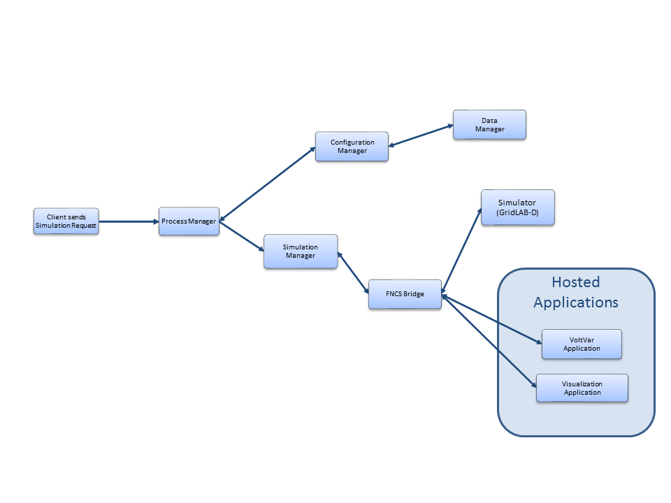
Process Manager - The workflow begins when a simulation request is sent to the request topic monitored by the Process Manager, the process manager gathers the necessary configurations from the Configuration Manager. Then sends the configuration to the simulation manager to run the simulation.
Configuration Manager - The configuration manager parses the request and builds the necessary configuration files. It also uses the data manager to pull the model data from the CIM database.
Data Manager - The data manager accesses the CIM database to build the model files used by the simulator.
Simulation Manager - The simulation manager launches the simulator and other required applications such as the FNCS bridge, FNCS, and the VoltVar application. It is in charge of managing the timing of the simulation and reporting output from the simulation out to the simulation status topic.
FNCS Bridge - Serves as input and output from the simulator to the rest of GridAPPS-D, receives initialization, timestep, update, and finalize requests from the simulation manager and other applications, such as voltvar. It also publishes output from the simulator on a pre-defined topic for the simulation manager and other applications to subscribe to.
Simulator - In this case GridLAB-D serves as the simulator.
Hosted Application - Applications can be developed to use the data generated by the simulation and submit feedback and updates to the simulator. Two examples of this have been developed in RC1, the VoltVar application and a vizualization application
Log Manager - Process Manager recieves a log message. It retrieves the username associated with the message and forwards the message and username to Log Manager. Log Manager writes the message on a file and if store_to_db key is true in log message then log manager calls the data manager to store the log message in the database.
CIM Documentation
This section summarizes the use of a reduced-order CIM [1] to support feeder modeling for the North American circuits and use cases considered in GridAPPS-D. The full CIM includes over 1100 tables in SQL, each one corresponding to a UML class, enumeration or datatype. RC1 used approximately 100 such entities, mapped onto 100+ tables in SQL. Subsequent versions of GridAPPS-D use a triple-store database, which is better suited for CIM [ref].
The CIM subset described here is based on iec61970cim17v23a_iec61968cim13v11, which formed the basis of a release candidate for CIM100. This candidate CIM100 already includes changes proposed from the GridAPPS-D project.
Class Diagrams for the Profile
Figure 1 through Figure 17 present the UML class diagrams generated from Enterprise Architect [2]. These diagrams provide an essential roadmap for understanding:
- How to ingest CIM XML from various sources into the database
- How to generate native GridLAB-D input files from the database
For those unfamiliar with UML class diagrams:
- Lines with an arrowhead indicate class inheritance. For example, in Figure 1, ACLineSegment inherits from Conductor, ConductingEquipment, Equipment and then PowerSystemResource. ACLineSegment inherits all attributes and associations from its ancestors (e.g., length), in addition to its own attributes and ancestors.
- Lines with a diamond indicate composition. For example, in Figure 1, Substations make up a SubGeographicalRegion, which then make up a GeographicRegion.
- Lines without a terminating symbol are associations. For example, in Figure 1, ACLineSegment has (through inheritance) a BaseVoltage, Location and one or more Terminals.
- Italicized names at the top of each class indicate the ancestor (aka superclass), in cases where the ancestor does not appear on the diagram. For example, in Figure 1, PowerSystemResource inherits from IdentifiedObject.
Please see GridAPPSD_RC4.eap [3] in the repository [4] on GitHub for the latest updates. The EnterpriseArchitect file includes a description of each class, attribute and association. It can also generate HTML documentation of the CIM, with more detail than provided here.
The diagrammed UML associations have a role and cardinality at each end, source and target. In practice, only one end of each association is profiled and implemented in SQL. In some cases, the figure captions indicate which end, but see the CIM profile for specific definitions, as described in the object diagram section. Usually, the end with 0..1 multiplicity is implemented instead of the end with 0..* or 1..* multiplicity.
Nearly every CIM class inherits from IdentifiedObject, from which we use two attributes:
- mRID is the “master identifier” that must be unique and persistent among all instances. It’s often used as the RDF resource identifier, and is often a GUID.
- Name is a human-readable identifier that need not be unique.
Figure 1 shows how equipment is organized into a Feeder. Each piece of Equipment has Terminals that connect at ConnectivityNodes, which represent the “buses”. Please note that in GridAPPS-D, we do not use TopologicalNode at all. In some CIM use cases, primary for transmission, the TopologicalNode coalesces ConnectivityNodes that are connected by buswork and closed switches into a single connection point. Instead, substation buswork models need to explicitly include the low-impedance branches and switches between ConnectivityNodes. We assume that modern distribution power flow solvers have no need of TopologicalNode.
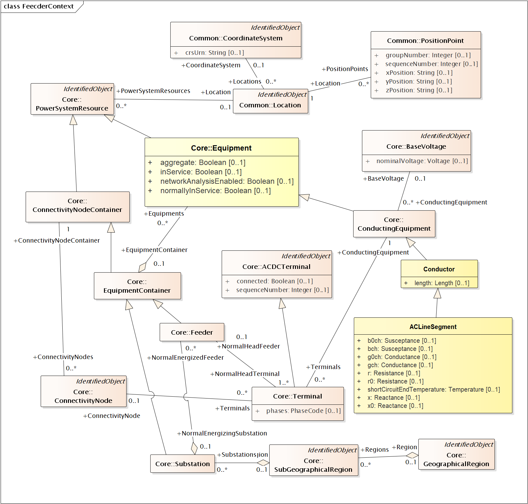
Figure 1: Placement of ACLineSegment into a Feeder. In GridAPPS-D, the Feeder is the EquipmentContainer for all power system components and the ConnectivityNodeContainer for all nodes. It’s energized from a Substation, which is part of a SubGeographicalRegion and GeographicalRegion for proper context with other CIM models. For visualization, ACLineSegment can be drawn from a sequence of PositionPoints associated via Location. The Terminals are free-standing; two of them will “reverse-associate” to the ACLineSegment as ConductingEquipment, and each terminal also has one ConnectivityNode. The Terminal:phases attribute is not used; instead, phases will be defined in the ConductingEquipment instances. The associated BaseVoltage:nominalVoltage attribute is important for many of the classes that don’t have their own rated voltage attributes, for example, EnergyConsumer.
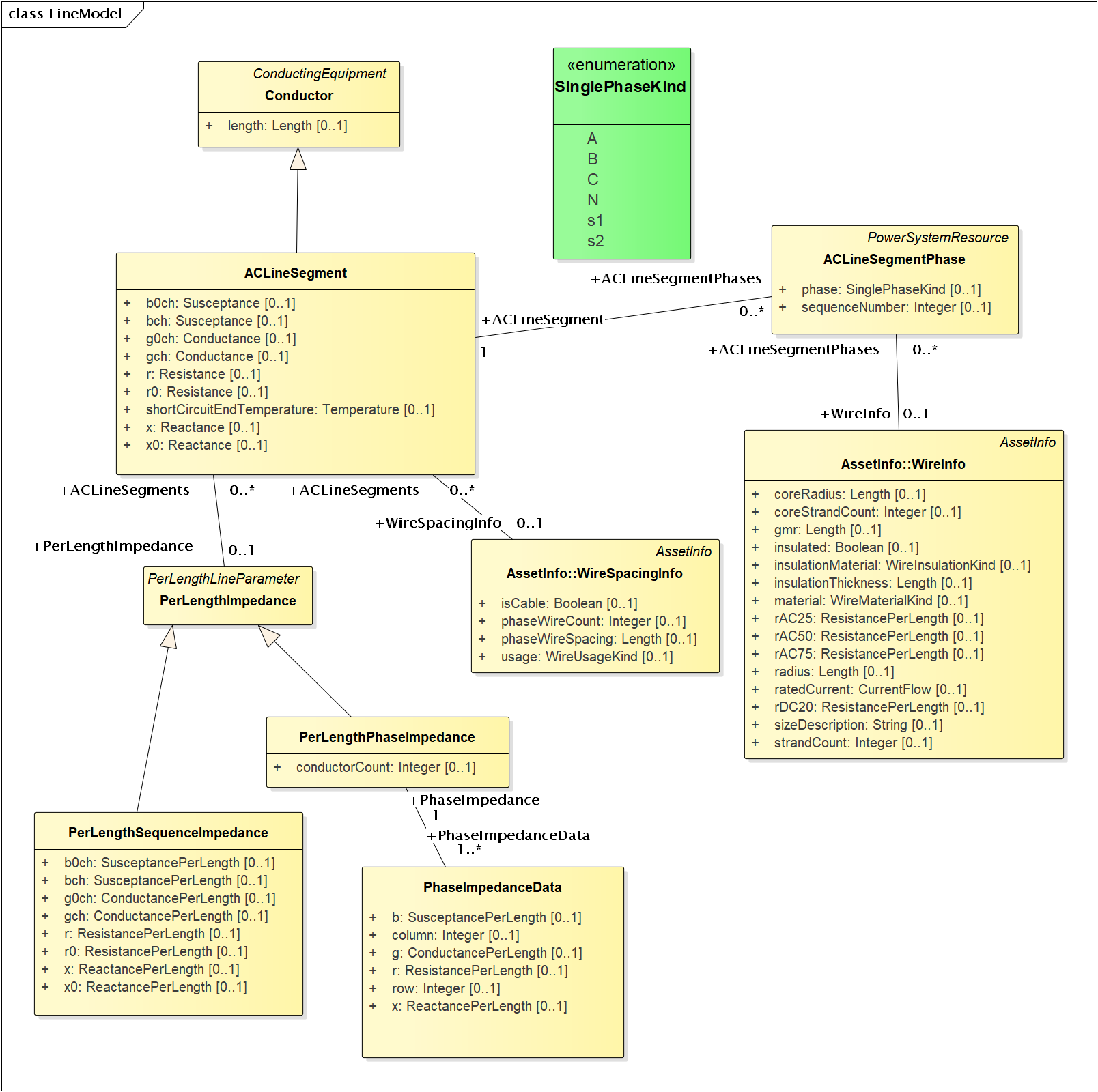
Figure 2: There are four different ways to specify ACLineSegment impedances. In all cases, Conductor:length is required. The first way is to specify the individual ACLineSegment attributes, which are sequence impedances and admittances, leaving PerLengthImpedance null. The second way is to specify the same attributes on an associated PerLengthSequenceImpedance, in which case the ACLineSegment attributes should be null. The third way is to associate a PerLengthPhaseImpedance, leaving the ACLineSegment attributes null. Only conductorCount from 1 to 3 is supported, and there will be 1, 3 or 6 reverse-associated PhaseImpedanceData instances that define the lower triangle of the Z and Y matrices per unit length. The row and column attributes must agree with ACLineSegmentPhase:sequenceNumber. The fourth way to specify impedance is by wire/cable and spacing data, by association to WireSpacingInfo and WireInfo. If there are ACLineSegmentPhase instances reverse-associated to the ACLineSegment, then per-phase modeling applies. There are several use cases for ACLineSegmentPhase: 1) single-phase or two-phase primary, 2) low-voltage secondary using phases s1 and s2, 3) associated WireInfo data where the WireSpacingInfo association exists, 4) assign specific phases to the matrix rows and columns in PerLengthPhaseImpedance. It is the application’s responsibility to propagate phasing through terminals to other components, and to identify any miswiring. (Note: this profile does not use WireAssemblyInfo, nor the fromPhase and toPhase attributes of PhaseImpedanceData.)
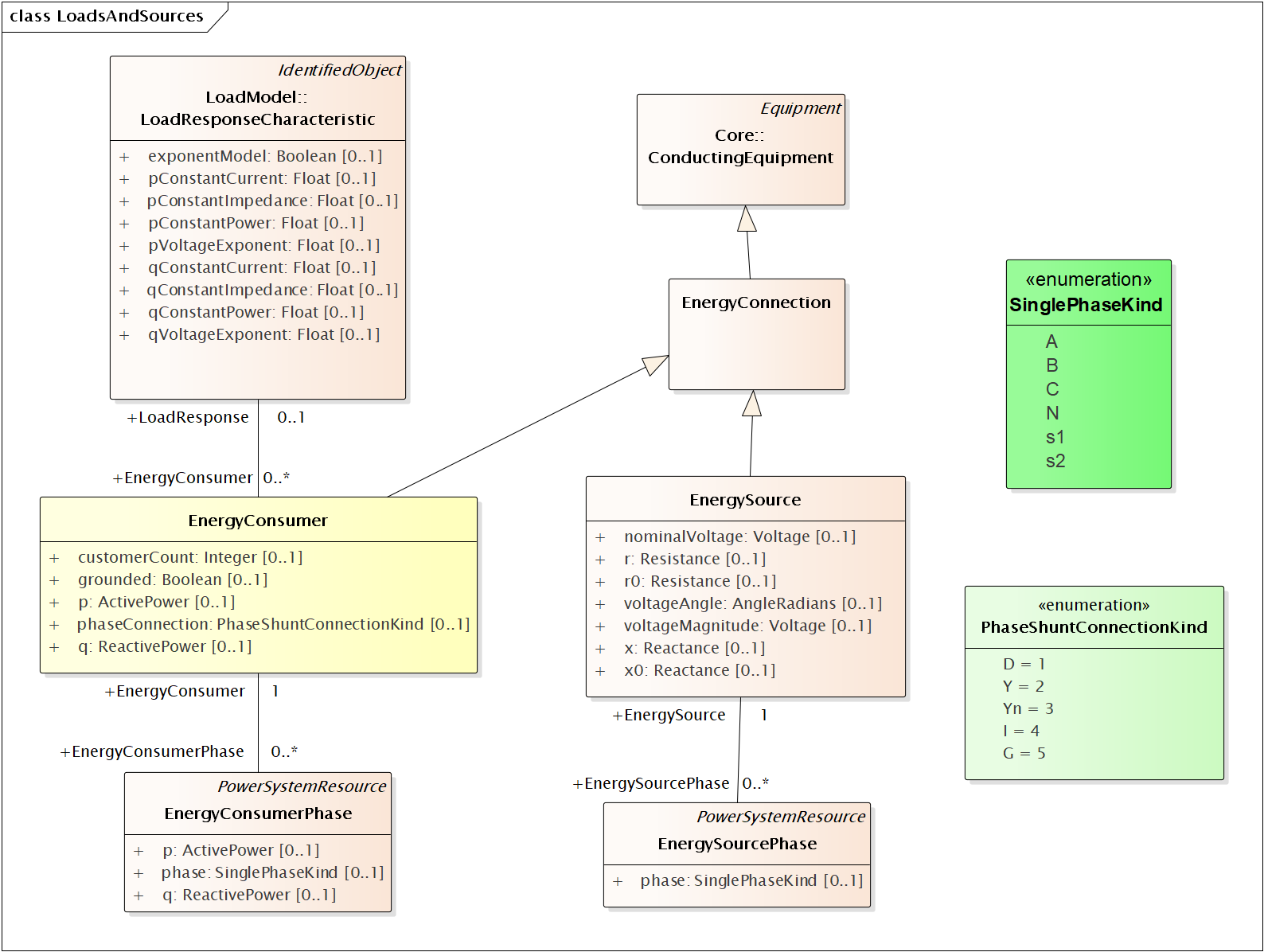
Figure 3: The EnergySource is balanced three-phase, balanced two-phase or single-phase Thevenin source. GridAPPS-D use a three-phase EnergySource to represent the transmission system. See Figures 13-14 for DER modeling. The EnergyConsumer is a ZIP load, possibly unbalanced, with an associated LoadResponse instance defining the ZIP coefficients. For three-phase delta loads, the phaseConnection is D and the three reverse-associated EnergyConsumerPhase instances will have phase=A for the AB load, phase=B for the BC load and phase=C for the AC load. A three-phase wye load may have either Y or Yn for the phaseConnection. Single-phase and two-phase loads, including secondary loads, should have phaseConnection=I (for individual).
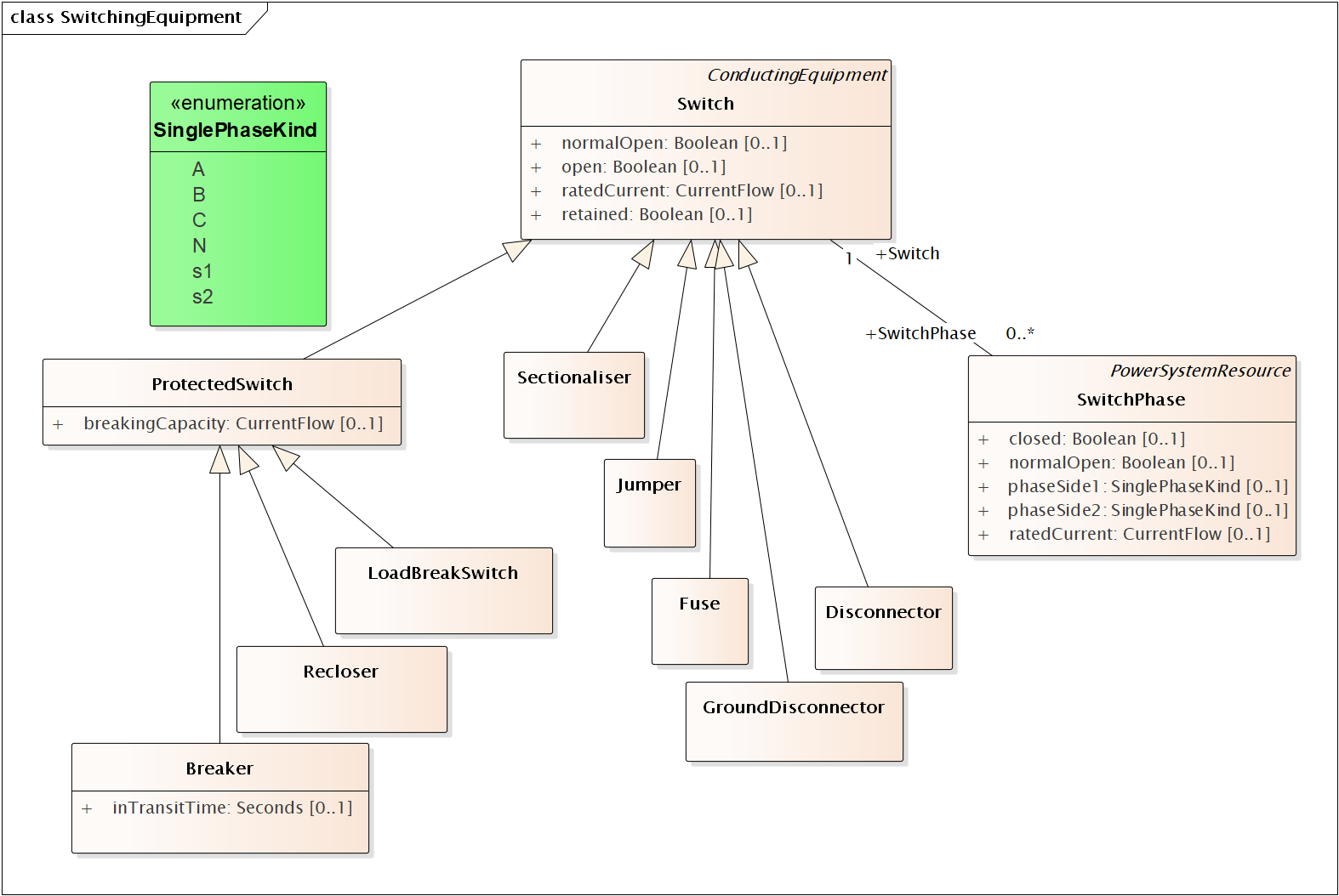
Figure 4: There are eight different kinds of Switch supported in the CIM, and all of them have zero impedance. They would all behave the same in power flow analysis, and all would require many more attributes than are defined in CIM to support protection analysis. The use cases for SwitchPhase include 1) single-phase, two-phase and secondary switches, 2) one or two conductors open in a three-phase switch or 3) transpositions, in which case phaseSide1 and phaseSide2 would be different. RatedCurrent may different among the phases, e.g., individual fuses on the same pole may have different ratings.
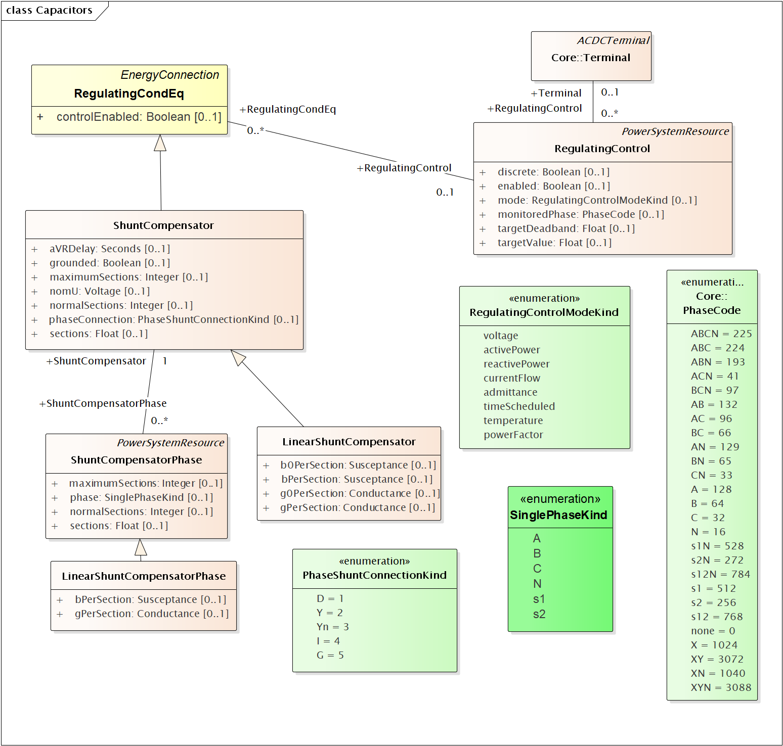
Figure 5: On the left, LinearShuntCompensator and LinearShuntCompensatorPhase define capacitor banks, in a way very similar to EnergyConsumer in Figure 3. The kVAR ratings must be converted to susceptance based on the nominal voltage, nomU. Note that aVRDelay is really a capacitor control parameter, to be used in conjunction with RegulatingControl on the right-hand side. The RegulatingControl associates to the controlled capacitor bank via RegulatingCondEq, and to the monitored location via Terminal. There is no support for a PT or CT ratio, so targetDeadband and targetValue have to be in primary volts, amps, vars, etc. Capacitor banks may _respond_ to any of the RegulatingControlModeKind choices, but it’s not expected that capacitor switching will successfully regulate to the targetValue.
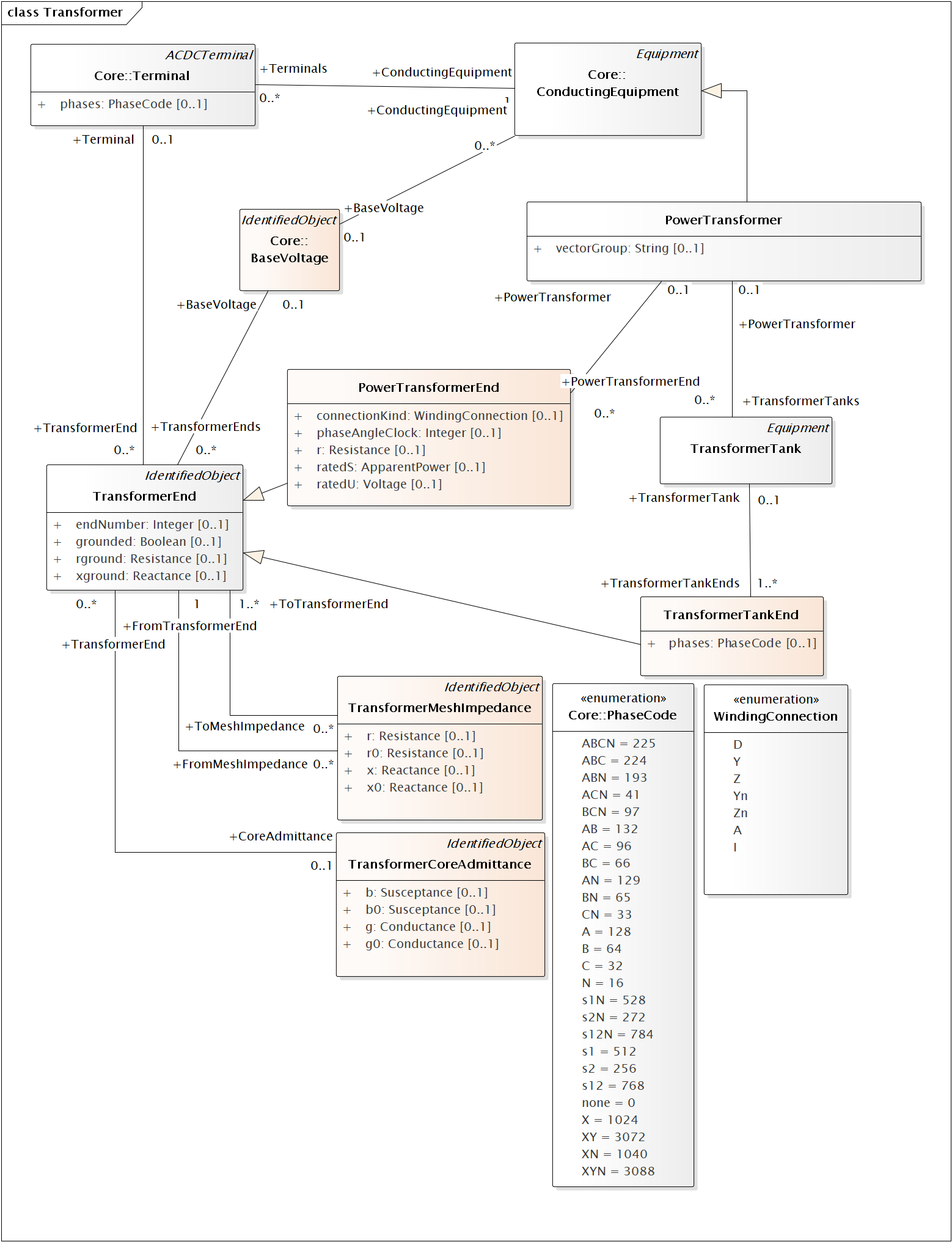
Figure 6: PowerTransformers may be modeled with or without tanks, and in both cases vectorGroup should be specified according to IEC transformer standards (e.g., Dy1 for many substation transformers). The case without tanks is most suitable for balanced three-phase transformers that won’t reference catalog data; any other case should use tank-level modeling. In the tankless case, each winding will have a PowerTransformerEnd that associates to both a Terminal and a BaseVoltage, and the parent PowerTransformer. The impedance and admittance parameters are defined by reverse-associated TransformerMeshImpedance between each pair of windings, and a reverse-associated TransformerCoreAdmittance for one winding. The units for these are ohms and siemens based on the winding voltage, rather than per-unit. WindingConnection is similar to PhaseShuntConnectionKind, adding Z and Zn for zig-zag connections and A for autotranformers. If the transformer is unbalanced in any way, then TransformerTankEnd is used instead of PowerTransformerEnd, and then one or more TransformerTanks may be used in the parent PowerTransformer. Some of the use cases are 1) center-tapped secondary, 2) open-delta and 3) EHV transformer banks. Tank-level modeling is also required if using catalog data, as described with Figure 9. (TransformerStarImpedance and several PowerTransformer attributes are not used. Star impedance attributes on PowerTransformerEnd and magnetic saturation attributes on TransformerEnd are not used.)
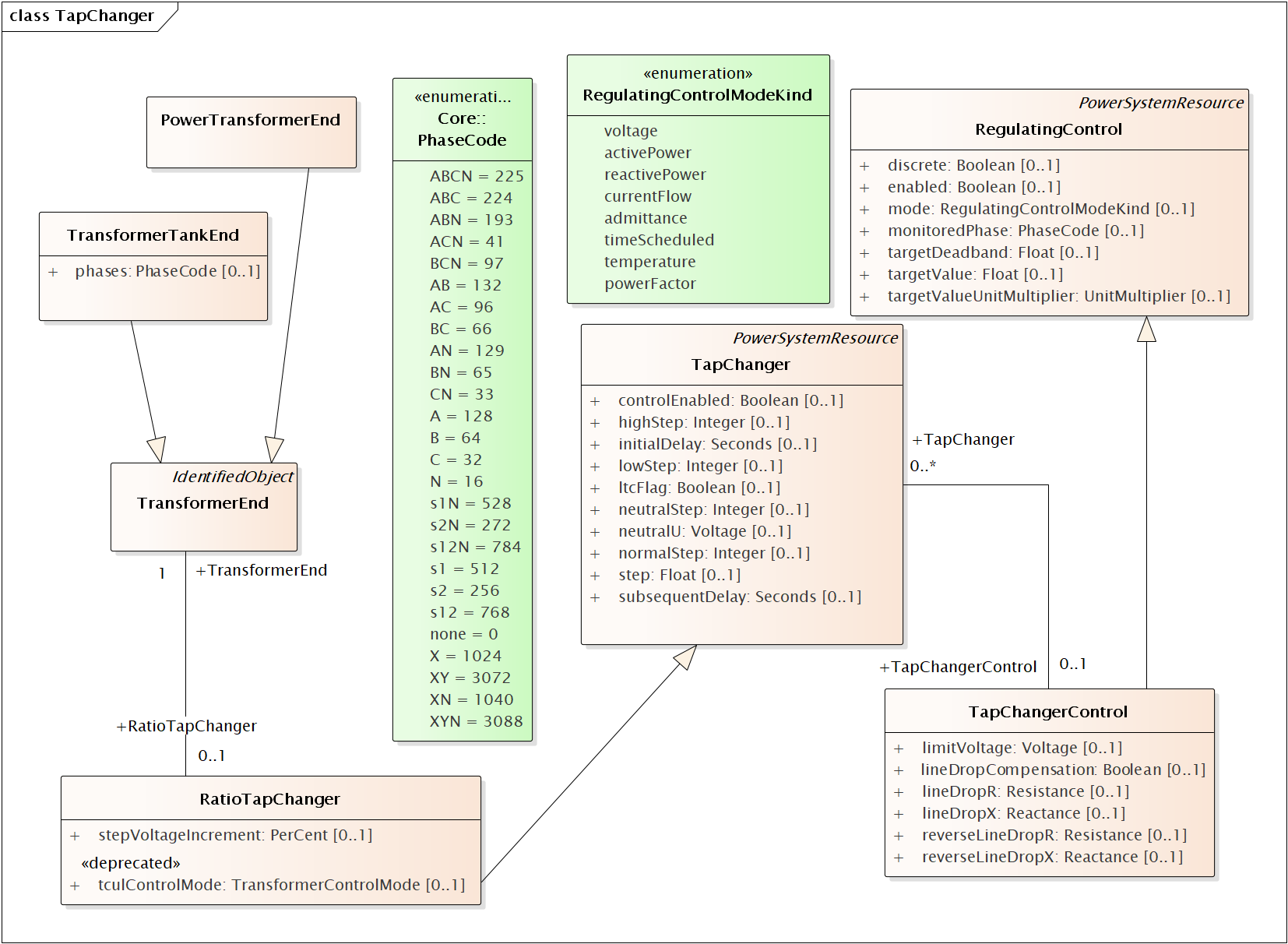
Figure 7: A RatioTapChanger can represent a transformer tap changer on the associated TransformerEnd. The RatioTapChanger has some parameters defined in a direct-associated TapChangerControl, which inherits from RegulatingControl some of the same attributes used in capacitor controls (Figure 5). Therefore, a line voltage regulator in CIM includes a PowerTransformer, a RatioTapChanger, and a TapChangerControl. The CT and PT parameters of a voltage regulator can only be described via the AssetInfo mechanism, described with Figure 8. The RegulationControl.mode must be voltage. (Note: RegulationSchedule, RatioTapChangerTable and PhaseTapChanger are not used.)
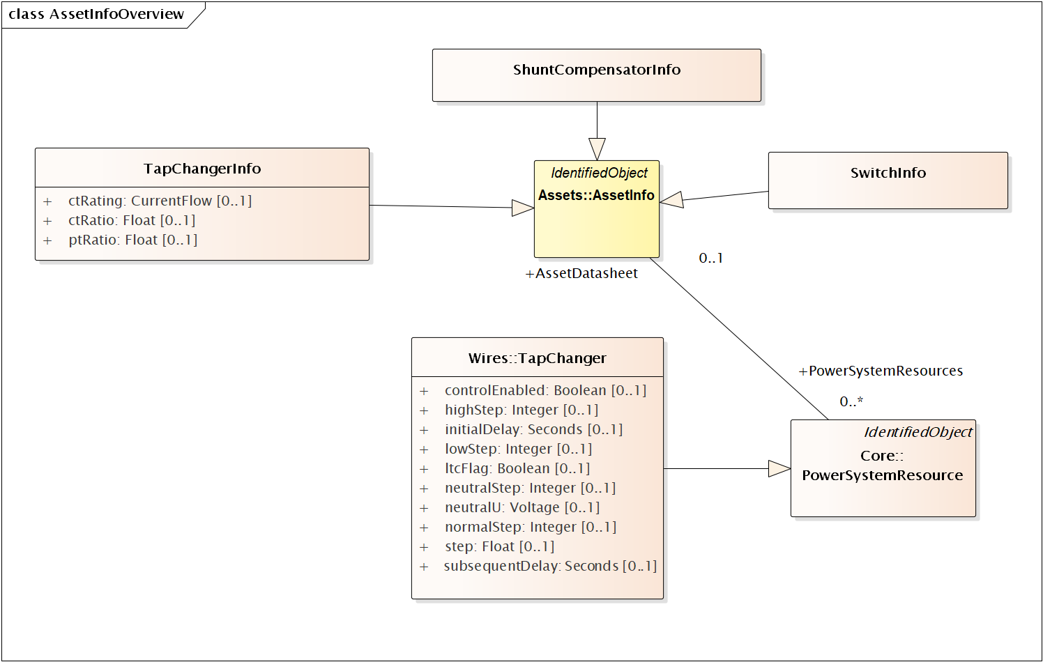
Figure 8: Many distribution software packages use the concept of catalog data, aka library data, especially for lines and transformers. We use the AssetInfo package to implement this in CIM. Here, the TapChangerInfo class includes the CT rating, CT ratio and PT ratio parameters needed for line drop compensator settings in voltage regulators. Catalog data is a one-to-many relationship. In this case, many TapChangers can share the same TapChangerInfo data, which saves space and provides consistency. Older versions of CIM had many-to-many catalog relationships, but now only one AssetDataSheet may be associated per Equipment. (Note: many datasheet attributes are not shown here and not yet used in GridAPPS-D).
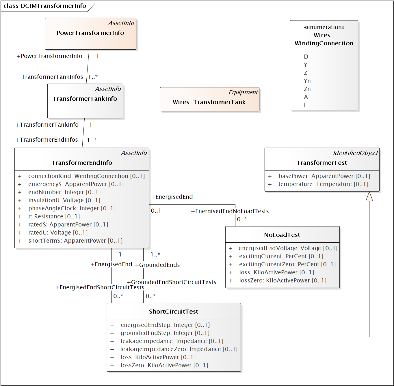
Figure 9: The catalog mechanism for transformers will associate a TransformerTank (Figure 6) with TransformerTankInfo (here), via the AssetDataSheet mechanism described in Figure 8. The PowerTransformerInfo collects TransformerTankInfo by reverse association, but it does not link with PowerTransformer. In other words, the physical tanks are cataloged because transformer testing is done on tanks. One possible use for PowerTransformerInfo is to help organize the catalog. It’s important that TransformerEndInfo:endNumber (here) properly match the TransformerEnd:endNumber (Figure 6). The shunt admittances are defined by NoLoadTest on a winding / end, usually just one such test. The impedances are defined by a set of ShortCircuitTests; one winding / end will be energized, and one or more of the others will be grounded in these tests. (OpenCircuitTest is not used, nor are the current, power and voltage attributes of ShortCircuitTest).
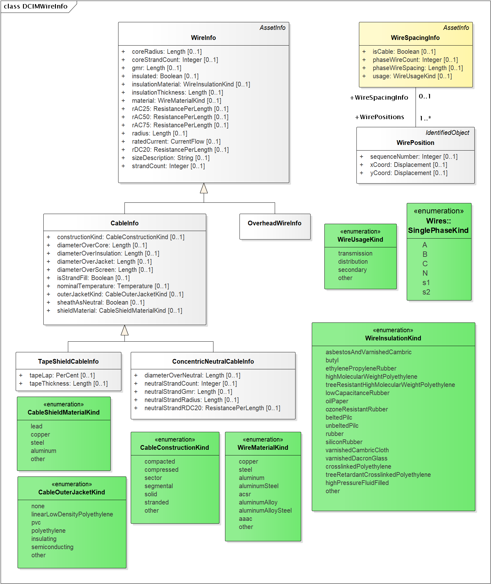
Figure 10: The catalog / library mechanism for ACLineSegment will have a WireSpacingInfo associated as in Figure 9. This will indicate whether the line is overhead or underground. phaseWireCount and phaseWireSpacing define optional bundling, so these will be 1 and 0 for distribution. The number of phase and neutral conductors is actually defined by the number of reverse-associated WirePosition instances. For example, a three-phase line with neutral would have four of them, sequenceNumber from 1 to 4. Each WirePosition’s phase is determined by the ACLineSegmentPhase with matching sequenceNumber, i.e., the phases need not be numbered in any particular order. On the left-hand side, concrete classes OverheadWireInfo, TapeShieldCableInfo and ConcentricNeutralCableInfo may be associated to ACLineSegmentPhase. It’s the application’s responsibility to calculate impedances from this data. In particular, soil resistivity and dielectric constants are not included in the CIM. Typical dielectric constant values might be defined for each WireInsulationKind.
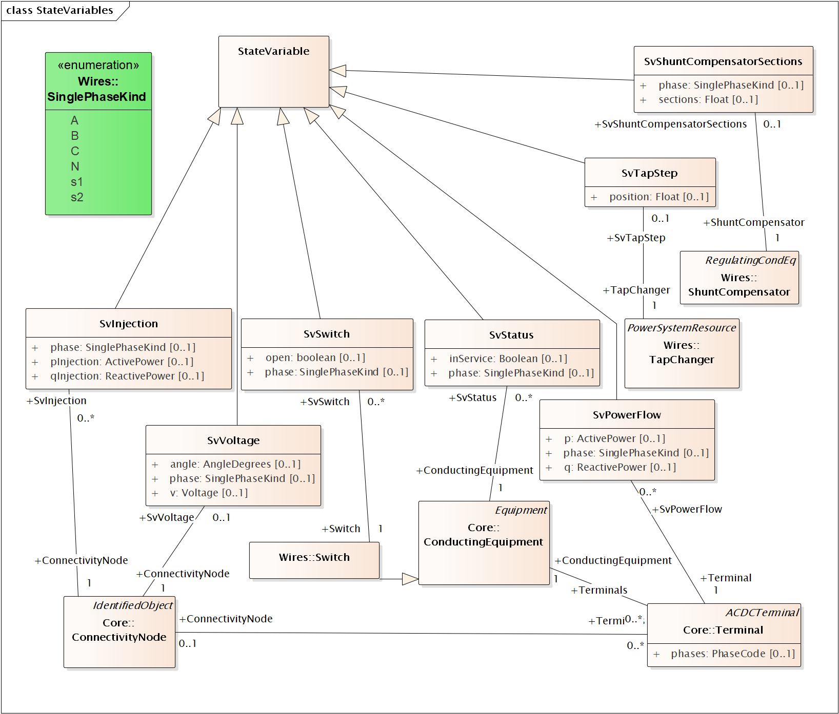
Figure 11: The CIM state variables package was designed to report power flow solution values on the distribution system. It could also report state estimator solutions as a special case of power flow solutions. Voltages are measured on ConnectivityNodes (i.e., not TopologicalNodes), power flows are measured at Terminals into the ConductingEquipment, step positions are measured on TapChangers, status is measured on ConductingEquipment, and on/off state is measured on ShuntCompensators for Switches. The “injections” have been included here, but there may not be a use case for them in distribution. On the other hand, solution values for current are very common in distribution system applications. These should be represented as SvPowerFlow values at the solved SvVoltage.
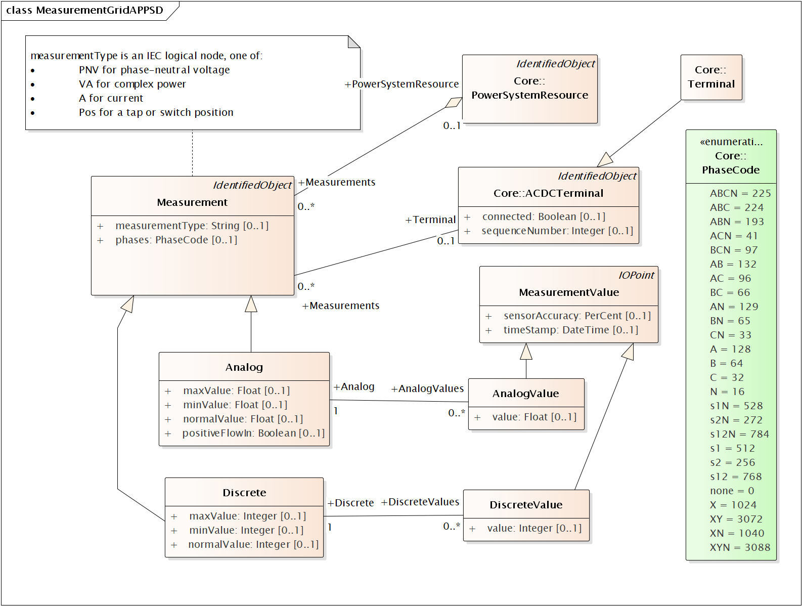
Figure 12: Measurements are defined in the Meas package. They differ from the state variables package, in that the values are measured here and not calculated or estimated. Each Measurement is associated to a PowerSystemResource, and in GridAPPS-D for now, also a Terminal that belongs to the same PowerSystemResource. (Non-electrical measurements, for example weather, would not have the Terminal). The measurementType is a string code from IEC 61850, with PNV, VA, A and POS currently supported. The Measurement has a name, mRID, and phases. In GridAPPS-D, each phase is measured individually so multi-phase codes like ABC should not be used. Pos measurements will be Discrete, for such things as tap position, switch position, or capacitor bank position. The others will be Analog, with magnitude and optional angle in degrees. Each MeasurementValue will have a timeStamp and mRID inherited from IdentifiedObject, so the values can be traced. (Note: IOPoint is a placeholder class with no attributes, inherting from IdentifiedObject. Further, it’s acceptable to supply an empty or short non-unique name for each MeasurementValue.)
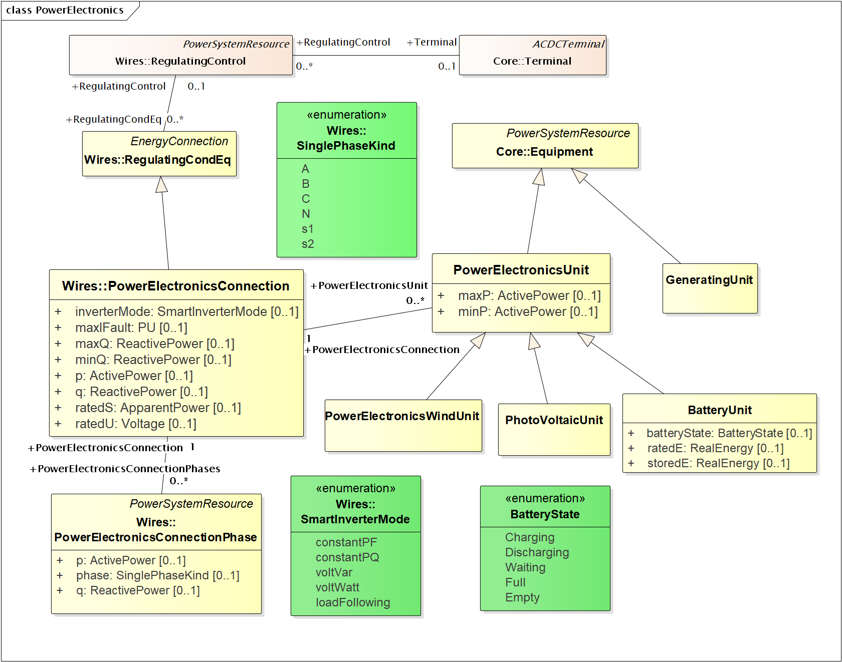
Figure 13: Power Electronics attributes are the minimum needed to support a time series power flow solution. For simple short-circuit calculations, maxIFault is provided as the inverter fault contribution in per-unit of rated current. When PowerElectronicsConnectionPhase is not present, the inverter is assumed to be balanced three-phase. The type of associated PowerElectronicsUnit determines whether the inverter is for solar or storage (wind is not currently used in GridAPPS-D). If the inverter employs a SmartInverterMode of voltVar, voltWatt or loadFollowing (storage only), then a Terminal should be associated through RegulatingControl, especially for loadFollowing. If the inverter will regulate its own Terminal, then the explicit Terminal association may not be needed. However, there are more attributes needed in CIM to define smart inverter functions. This might be done in harmonization with IEC 61850, which does define smart inverter function parameters. The existing CIM RegulatingControl attributes are probably not applicable, so they have been hidden in Figure 13.
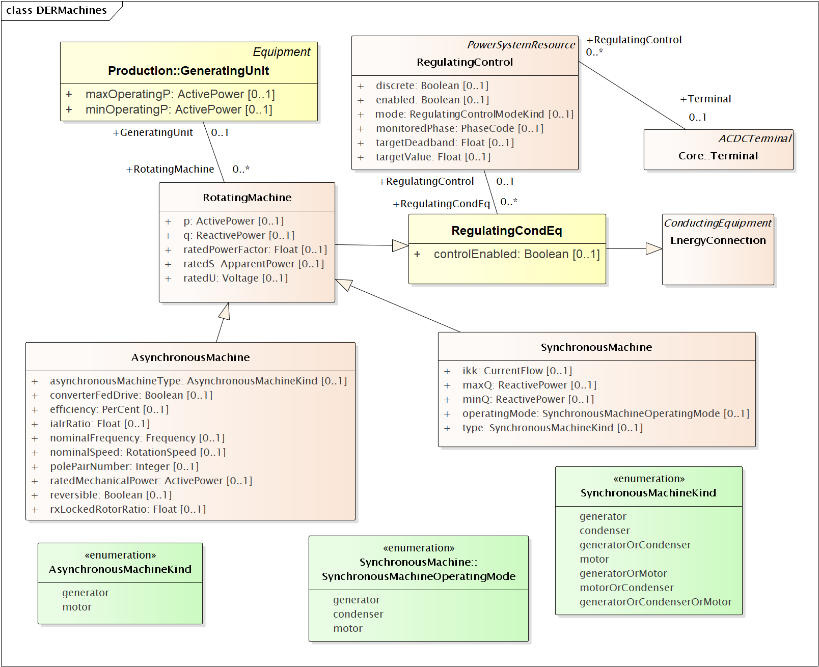
Figure 14: Rotating Machines are three-phase balanced, either synchronous or asynchronous. The SynchronousMachine ikk attribute and most of the AsynchronousMachine attributes are provided to support short-circuit calculations according to IEC 60909. The GeneratingUnit class is needed to define minimum and maximum power limits. In the full CIM, GeneratingUnit is an abstract class with descendants HydroUnit, ThermalUnit and NuclearUnit, but in GridAPPS-D we don’t currently distinguish between those types. If the SynchronousMachine regulates voltage, then the RegulatingControl (with attribute values) and Terminal associations need to be provided.
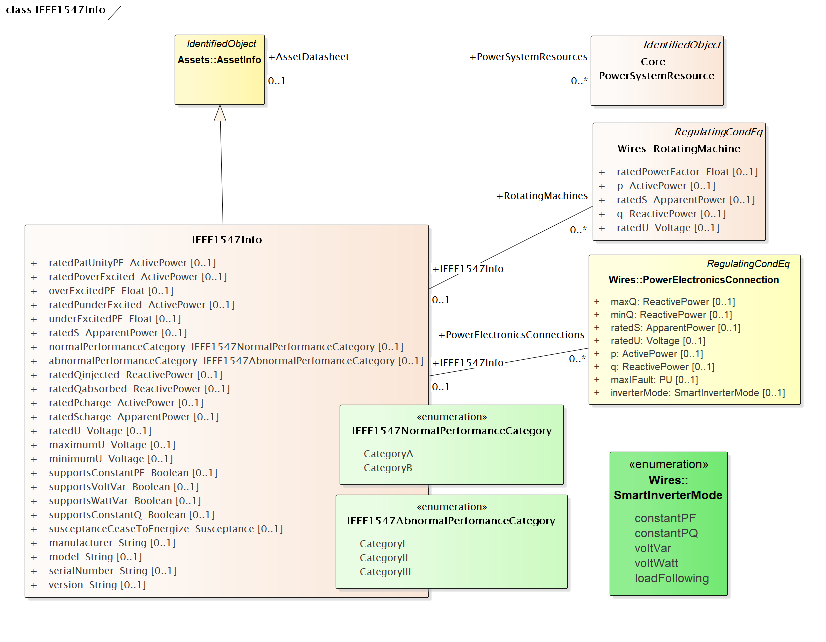
Figure 15: The IEEE1547Info class describes nameplate information, including ratings, which shall be available for DER that complies with IEEE Std. 1547-2018. Both inverters (Figure 13) and rotating machines (Figure 14) can reference this class for nameplate information in the network model. Preliminary values for these attributes would be available from an application to interconnect DER, and then updated as the project moves through commissioning to operational status.
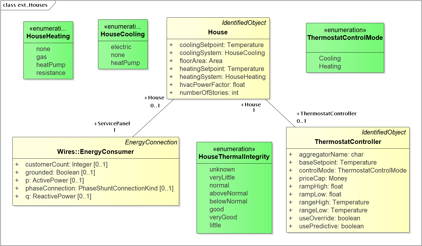
Figure 16: Houses are used to create 2nd-order thermal models of the building envelope, with internal ThermostatController and heating/cooling systems. The purpose is to introduce realistic load stochastic behaviors that are independent from and faster-moving than data typically available to an electric utility. To enable repeatable simulations, the House data structures have been defined here as a CIM extension. The House must be attached to one EnergyConsumer that incorporates other end-use loads, and connects to the distribution system. The House attributes are the minimum necessary to define a GridLAB-D house model, and during simulation, the house heating/cooling system will add to the ServicePanel loads. Therefore, the application should reduce the nominal value of EnergyConsumer.p in order to “make room” for the heating/cooling load that will switch on and off, responding to the ThermostatController and the weather. The ThermostatController contains the minimum attributes needed for PNNL’s double-ramp, double-auction market mechanism. In the future, this will be harmonized with CIM market structures in the 62235 package.
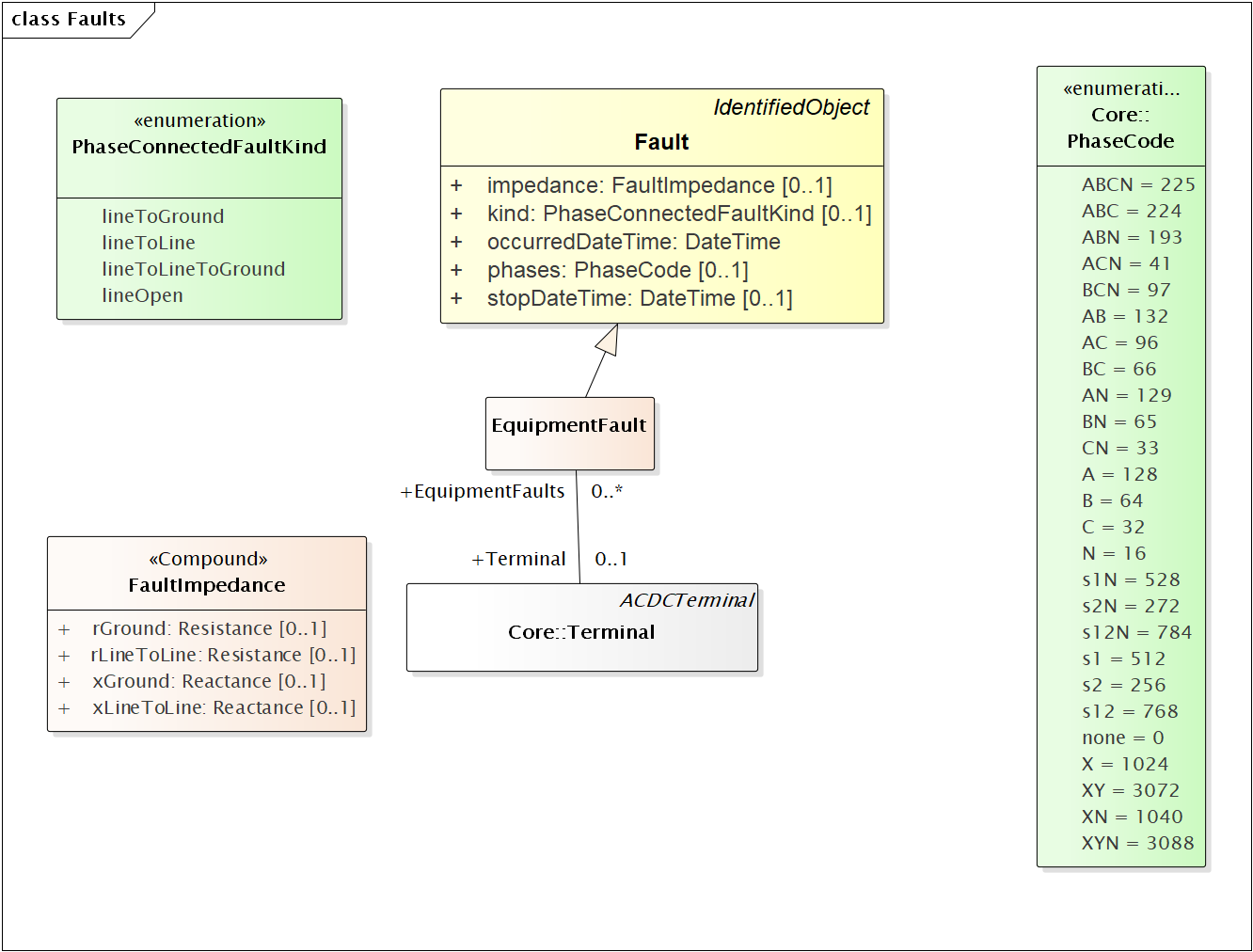
Figure 17: Faults include open conductors and short circuits (optionally including ground) on any combination of phases. In GridAPPS-D, every Fault will be an EquipmentFault associated to a Terminal (i.e., we are not using LineFault, which requires a lengthFromTerminal1 attribute). The occurredDateTime supports the scripting of fault sequences. The stopDateTime is optional. If provided, it will be the time at which a sustained fault has been repaired. If not provided, then the fault is temporary and will clear itself as soon as it’s been deenergized.
Typical Queries
These queries focus on requirements of the first volt-var application.
- Capacitors (Figure 5, Figure 18, Figure 19, Figure 20)
- Create a list of capacitors with bus name (Connectivity Node in Figure 1), kVAR per phase, control mode, target value and target deadband
- For a selected capacitor, update the control mode, target value, and target deadband
- Regulators (Figure 7, Figure 8, Figure 18, Figure 35)
- List all transformers that have a tap changer attached, along with their bus names and kVA sizes
- Given a transformer that has a tap changer attached, list or update initialDelay, step, subsequentDelay, mode, targetDeadband, targetValue, limitVoltage, lineDropCompensation, lineDropR, lineDropX, reverseLineDropR and reverseLineDropX
- Transformers (Figure 6, Figure 9)
- Given a bus name or load (Figure 3), find the transformer serving it (Figure 22, Figure 25)
- Find the substation transformer, defined as the largest transformer (by kVA size and or highest voltage rating)
- List the transformer catalog (Figure 9, Figure 26) with name, highest ratedS, list of winding ratedU in descending order, vector group (https://en.wikipedia.org/wiki/Vector_group used with connectionKind and phaseAngleClock), and percent impedance
- List the same information as in item c, but for transformers
(Figure 6) and also retrieving their bus names. Note that a
transformer can be defined in three ways
- Without tanks, for three-phase, multi-winding, balanced transformers (Figure 22 and Figure 23).
- With tanks along with TransformerTankInfo (Figure 9) from a catalog of “transformer codes”, which may describe balanced or unbalanced transformers. See Figure 25 and Figure 26.
- With tanks for unbalanced transformers, and TransformerTankInfo created on-the-fly. See Figure 25 and Figure 26.
- Given a transformer (Figure 6), update it to use a different catalog entry (TransformerTankInfo in Figure 9)
- Lines (Figure 2, Figure 10, Figure 18)
- List the line and cable catalog entries that meet a minimum ratedCurrent and specific WireUsageKind. For cables, be able to specify tape shield vs. concentric neutral, the WireInsulationKind, and a minimum insulationThickness. (Figure 33)
- Given a line segment (Figure 2) update to use a different linecode (Figure 10, Figure 32)
- Given a bus name, list the ACLineSegments connected to the bus, along with the length, total r, total x, and phases used. There are four cases as noted in the caption of Figure 2, and see Figure 29 through Figure 32.
- Given a bus name, list the set of ACLineSegments (or PowerTransformers and Switches) completing a path from it back to the EnergySource (Figure 3). Normally, the applications have to build a graph structure in memory to do this, so it would be very helpful if a graph/semantic database can do this.
- Voltage and other measurements (Figure 1, Figure 11)
- Given a bus, attach a voltage solution point (SvVoltage, Figure 36)
- List all voltage solution points and their buses, and for each bus, list the phases actually present
- For tap changer position (SvTapStep, Figure 37), attach and list values as in items a and b
- For capacitor switch status (SvShuntCompensatorSections, Figure 38), attach and list values as in items a and b
- Loads (Figure 3, Figure 34)
- Given a bus name, list and total all of the loads connected by phase, showing the total p and q, and the composite ZIP coefficients
- Switching (Figure 4, Figure 28)
- Given a bus name, trace back to the EnergySource and list the switches encountered, grouped by type (i.e. the leaf class in Figure 4). Also include the ratedCurrent, breakingCapacity if applicable, and open/close status. If SwitchPhase is used, show the phasing on each side and the open/close status of each phase.
- Given switch, toggle its open/close status.
Object Diagrams for Queries
This section contains UML object diagrams for the purpose of illustrating how to perform typical queries and updates. For those unfamiliar with UML object diagrams:
- Each object will be an instance of a class, and more than one instance of a class can appear on the diagram. For example, Figure 18 shows two ConnectivityNode instances, one for each end of a ConductingEquipment.
- The object name (if specified and important) appears before the colon (:) above the line, while the UML class appears after the colon. Every object in CIM will have a unique ID, and a name (not necessarily unique), even if not shown here.
- Some objects may be shown with run-time state below the line. These are attribute value assignments, drawn from those available in the UML class or one of the class ancestors. The object may have more attribute assignments, but only those directly relevant to the figure captions are shown in the diagrams of this section.
- Object associations are shown with solid lines, role names, and multiplicities similar to the UML class diagrams. One important difference is that only one way of navigating a particular association will be defined in the profile. For example, the lower left corner of Figure 1 shows a two-way link between Terminal and ConnectivityNode in the UML class diagram. However, Figure 18 shows that only one direction has been defined in the profile. Each Terminal has a direct reference to its corresponding ConnectivityNode. In order to navigate the reverse direction from ConnectivityNode to Terminal, some type of conditional query would be required. In other words, the object diagrams in this section indicate which associations can actually be used in GridAPPS-D.
- In some cases, the multiplicities on the object diagrams are more restrictive than on the class diagrams, due to profiling. For example, EnergyConsumer and ShuntCompensator must have exactly one Terminal, not 1..*.
The object diagrams are intended to help you break down the CIM queries into common sub-tasks. For example, query #1 works with capacitors. It’s always possible to select a capacitor (aka LinearShuntCompensator) by name. In order to find the capacitor at a bus, say “bus1” in Figure 12, one would retrieve all Terminals having a ConnectivityNode reference to “bus1”. Each of those Terminals will have a ConductingEquipment reference, and you want the Terminal(s) for which that reference is actually a LinearShuntCompensator. In this CIM profile, only leaf classes (e.g. LinearShuntCompensator) will be instantiated, never base classes like ConductingEquipment. There can be more than one capacitor at a bus, more than one load, more than one line, etc.
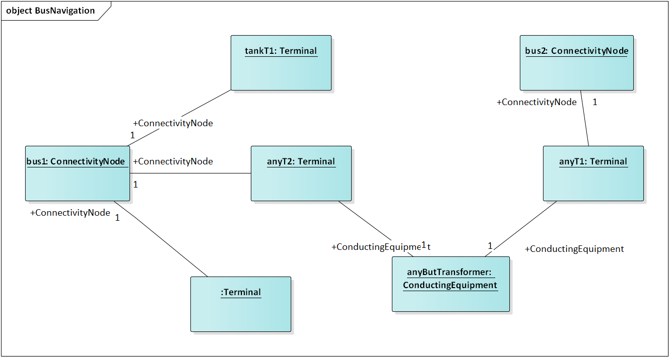
Figure 18: In order to traverse buses and components, begin with a ConnectivityNode (left). Collect all terminals referencing that ConnectivityNode; each Terminal will have one-to-one association with ConductingEquipment, of which there are many subclasses. In this example, the ConductingEquipment has a second terminal referencing the ConnectivityNode called bus2. There are applications for both Depth-First Search (DFS) and Bread-First Search (BFS) traversals. Note 1: the Terminals have names, but these are not useful. In some cases, the Terminal sequenceNumber attribute is needed to clearly identify ends of a switch. Note 2: in earlier versions of GridAPPS-D, we had one-to-one association of TopologicalNode and ConnectivityNode, but these are no longer necessary. Note 3: transformers are subclasses of ConductingEquipment, but we traverse connectivity via transformer ends (aka windings). This is illustrated later.
In order to find capacitors (or anything else) associated with a particular “feeder”, Figure 19 shows that you would query for objects having EquipmentContainer reference to the Feeder object. In GridAPPS-D, we only use Feeder for equipment container in CIM, and this would correspond to one entire GridLAB-D model. There is also a BaseVoltage reference that will have the system nominal voltage for the capacitor’s location. However, in order to work with equipment ratings you should use ratedS and ratedU attributes where they exist, particularly for capacitors and transformers. These attributes are often slightly different than the “system voltage”. Most of the attribute units in CIM are SI, with a few exceptions like percent and kW values on transformer test sheets (i.e., CIM represents the test sheet, not the equipment).
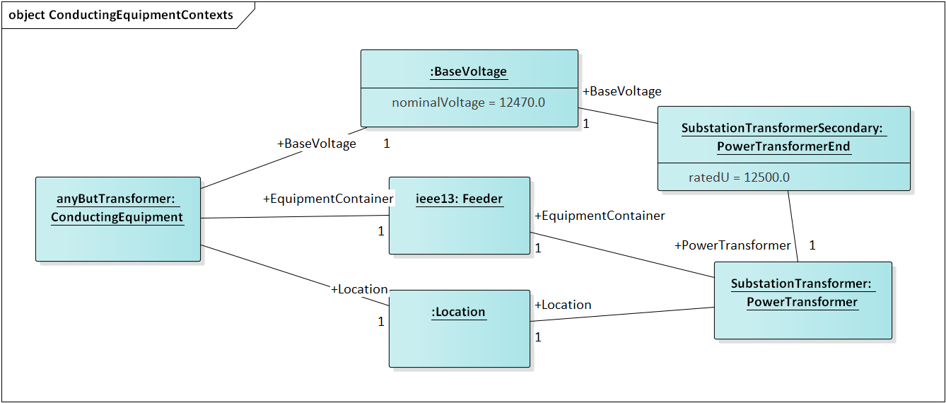
Figure 19: All conducting equipment lies within an EquipmentContainer, which in GridAPPS-D, will be a Feeder object named after the feeder. It also has reference to a BaseVoltage, which is typically one of the ANSI preferred system voltages. Power transformers are a little different, in that each winding (called “end” in CIM) has reference to a BaseVoltage. Note that equipment ratings come from the vendor, and in this case ratedU is slightly different from nominalVoltage. All conducting equipment has a Location, which contains XY coordinates (see Figure 1). The Location is useful for visualization, but is not essential for a power flow model.
Completing the discussion of capacitors, Figure 20 provides two examples for single-phase, and three-phase with local voltage control. As shunt elements, capacitors have only one Terminal instance. Loads and sources have one terminal, lines and switches have two terminals, and transformers have two or more terminals. Examples of all those are shown later. In Figure 20, the capacitor’s kVAR rating will be based on its nameplate ratedU, not the system’s nominalVoltage.
Often, the question will arise “what phases exist at this bus?”.There is no phasing explicitly associated with a ConnectivityNode, and we don’t use the Terminal phases attribute in preference to the “wires phase model” classes. For example, thephases at a line segment terminal can always be obtained from the ACLineSegmentPhase instances. To answer the question about bus phasing, we’d have to query for all ConductingEquipment instances having Terminals connected to that bus, as in Figure 18. The types of ConductingEquipment that may have individual phases include LinearShuntCompensators (Figure 20), ACLineSegments, PowerTransformers (via TransformerEnds), EnergyConsumers, EnergySources, PowerElectronicsConnections, and descendants of Switch. If the ConductingEquipment has such individual phases, then add those phases to list of phases existing at the bus. If there are no individual phases, then ABC all exist at the bus. Note this doesn’t guarantee that all wiring to the bus is correct; for example, you could still have a three-phase load served by only a two-phase line, which would be a modeling error. In Figure 20, we’d find phase C at Bus611 and phases ABC at Bus675. Elsewhere in the model, there should be ACLineSegments, PowerTransformers or Switch descendants delivering phase C to Bus611, all three phases ABC to Bus675.
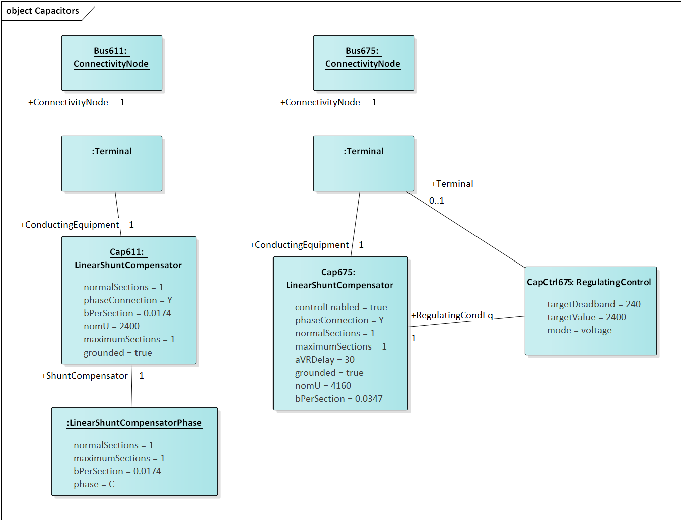
Figure 20: Capacitors are called LinearShuntCompensator in CIM. On the left, a 100 kVAR, 2400 V single-phase bank is shown on phase C at bus 611. bPerSection = 100e3 / 2400^2 [S], and the bPerSection on LinearShuntCompensatorPhase predominates; these values can differ among phases if there is more than one phase present. On the right, a balanced three-phase capacitor is shown at bus 675, rated 300 kVAR and 4160 V line-to-line. We know it’s balanced three phase from the absence of associated LinearShuntCompensatorPhase objects. bPerSection = 300e4 / 4160^2 [S]. This three-phase bank has a voltage controller attached with 2400 V setpoint and 240 V deadband, meaning the capacitor switches ON if the voltage drops below 2280 V and OFF if the voltage rises above 2520 V. These voltages have to be monitored line-to-neutral in CIM, with no VT ratio. In this case, the control monitors the same Terminal that the capacitor is connected to, but a different conducting equipment’s Terminal could be used. The control delay is called aVRDelay in CIM, and it’s an attribute of the LinearShuntCompensator instead of the RegulatingControl. It corresponds to “dwell time” in GridLAB-D.
Figure 21 through Figure 26 illustrate the transformer query tasks, plus Figure 35 for attached voltage regulators. The autotransformer example is rated 500/345/13.8 kV and 500/500/50 MVA, for a transmission system. The short circuit test values are ZHL=10%, ZHT=25% and ZLT=30%. The no-load test values are 0.05% exciting current and 0.025% no-load losses. These convert to r, x, g and b in SI units, from ZLT= Urated* Urated/ Srated, where Sratedand Uratedare based on the “from” winding (aka end). The same base quantities would be used to convert r, x, g and b back to per-unit or percent. The open wye – open delta impedances are already represented in percent or kW, from the test reports.
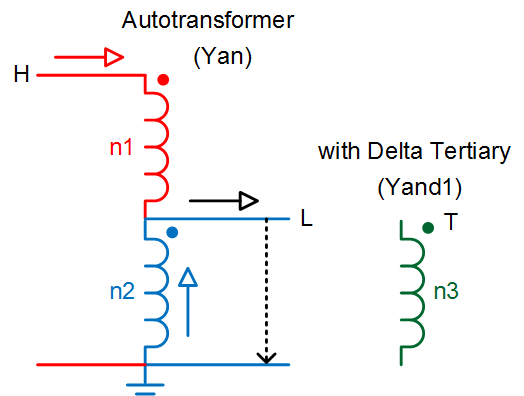
Figure 21: Autotransformer with delta tertiary winding acts like a wye-wye transformer with smaller delta tertiary. The vector group would be Yynd1 or Yyd1. For analyses other than power flow, it can be represented more accurately as the physical series (n1) – common (n2) connection, with a vector group Yand1. In either case, it’s a three-winding transformer.
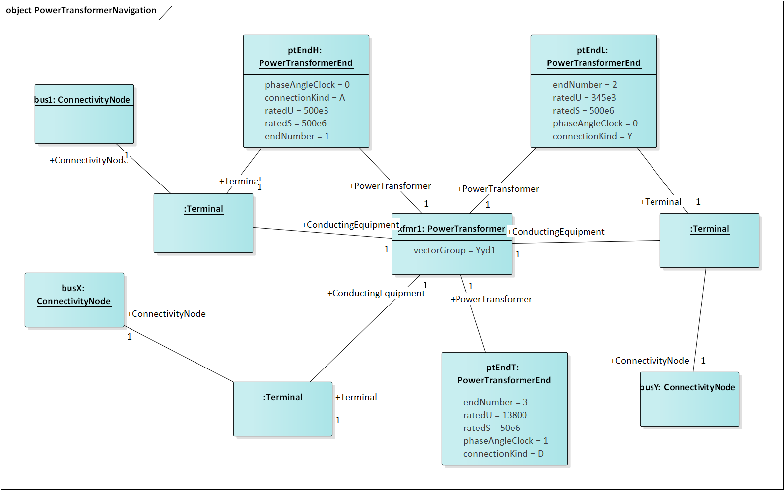
Figure 22: A three-winding autotransformer is represented in CIM as a PowerTransformer with three PowerTransformerEnds, because it’s balanced and three-phase. The three Terminals have direct ConductingEquipment references to the PowerTransformer, so you can find it from bus1, busX or busY. However, each PowerTransformerEnd has a back-reference to the same Terminal, and it’s own reference to BaseVoltage (Figure 13); that’s how you link the matching buses and windings, which must have compatible voltages. Terminals have a sequenceNumber, but the PowerTransformerEnd’s endNumber is what establishes correct linkage to catalog data as discussed later. By convention, ends with highest ratedU have the lowest endNumber, and endNumber establishes that end’s place in the vectorGroup.
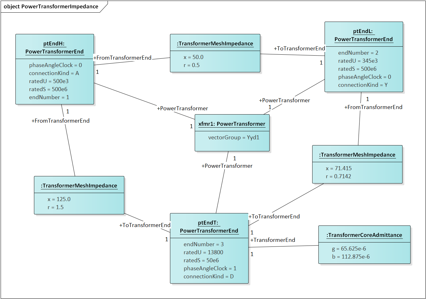
Figure 23: Power transformer impedances correspond to the three-winding autotransformer example of Figure 15 and Figure 16. There are three instances of TransformerMeshImpedance connected pair-wise between the three windings / ends. The x and r values are in Ohms referred to the end with highest ratedU in that pair. There is just one TransformerCoreAdmittance, usually attached to the end with lowest ratedU, and the attribute values are Siemens referred to that end’s ratedU.
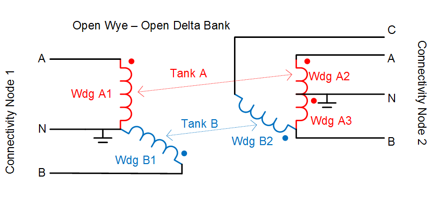
Figure 24: Open wye - open delta transformer banks are used to provide inexpensive three-phase service to loads, by using only two single-phase transformers. This is an unbalanced transformer, and as such it requires tank modeling in CIM. Physically, the two transformers would be in separate tanks. Note that Tank A is similar to the residential center-tapped secondary transformer, except the CIM phases for the secondary would include s1 and s2 instead of A and B.
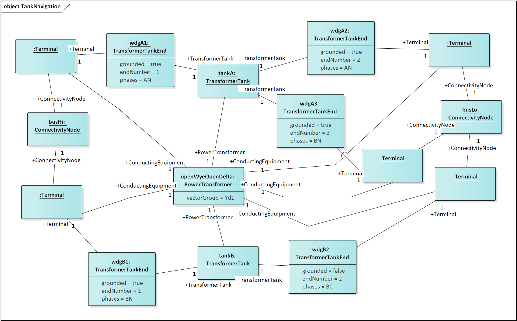
Figure 25: Unbalanced PowerTransformer instances comprise one or more TransformerTanks, which own the TransformerTankEnds. Through the ends, wdgHi collects phases ABN and busLo collects phases ABCN. Typically, phase C will also exist at wdgHi, but this transformer doesn’t require it. We still assign vectorGroup Yd1 to the supervising PowerTransformer, as this is the typical case. The modeler should determine that. By comparison to Figure 24, there is a possible ambiguity in how endA3 represents the polarity dot at the neutral end of Wdg A3. An earlier CIM proposal would have assigned phaseAngleClock = 6 on wdgA3, but the attribute was removed from TransformerTankEnd. It may not be possible to infer the correct winding polarities from the vectorGroup in all cases. There is a phaseAngleClock attribute on TransformerTankEndInfo, but that represents a shelf state of the tank, not necessarily connections in the field. Therefore, it may be necessary to propose the phaseAngleClock attribute for TransformerTankEnd.
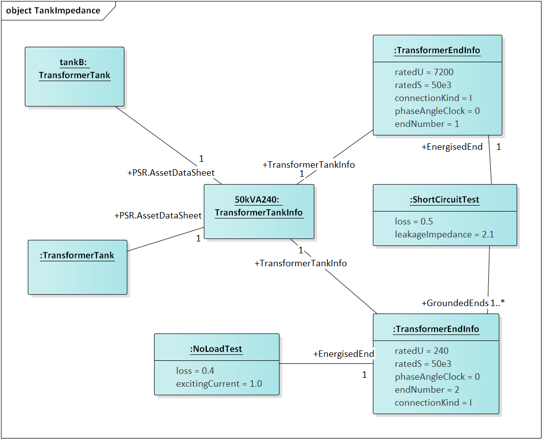
Figure 26: This Asset catalog example defines the impedances for Tank B of the open wye – open delta bank. This is a 50 kVA, 7200 / 240 V single-phase transformer. It has 1% exciting current and 0.4 kW loss in the no-load test, plus 2.1% reactance and 0.5 kW loss in the short-circuit test. A multi-winding transformer could have more than one grounded end in a short-circuit test, but this is not common. The catalog data is linked with an AssetDataSheet association shown to the left. Furthermore, endNumber on the TransformerEndInfo has to match endNumber on the TransformerTankEnd instances associated to Tank B. Instead of catalog information, we could have used mesh impedance and core admittance as in Figure 18, but we’d have to convert the test sheets to SI units and we could not share data with other TransformerTank instances, both of which are inconvenient.
Figure 27 through Figure 33 illustrate the query tasks for ACLineSegments and Switches, which will define most of the circuit’s connectivity. The example sequence impedances were based on Z1 = 0.1 + j0.8 Ω/mile and Z0 = 0.5 + j2.0 Ω /mile. For distribution systems, use of the shared catalog data is more common, either pre-calculated matrix (Figure 31) or spacing and conductor (Figure 32 and Figure 33). In both cases, impedance calculation is outside the scope of CIM (e.g. GridLAB-D internally calculates line impedance from spacing and conductor data).
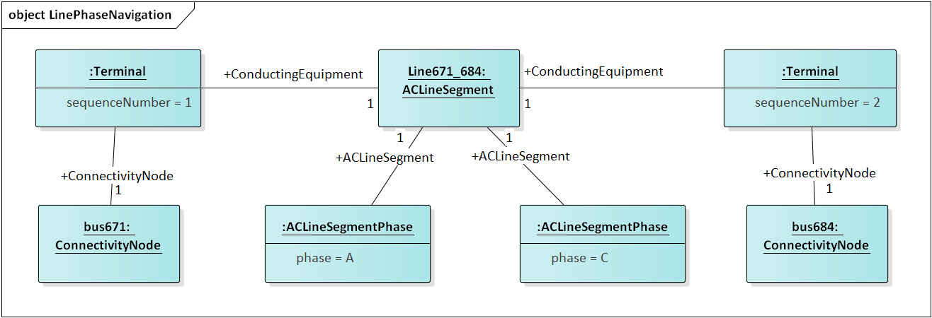
Figure 27: An ACLineSegment with two phases, A and C. If there are no ACLineSegmentPhase instances that associate to it, assume it’s a three-phase ACLineSegment. This adds phases AC to bus671 and bus684.
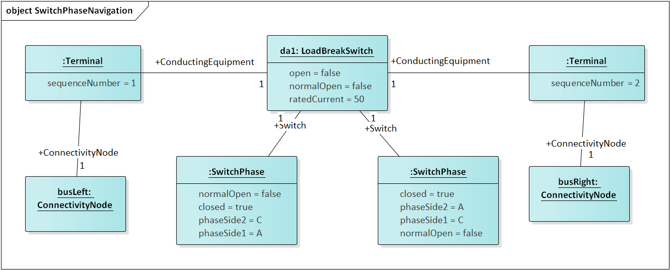
Figure 28: This 50-Amp load break switch connects phases AC between busLeft and busRight. Without associated SwitchPhase instances, it would be a three-phase switch. This switch also transposes the phases; A on side 1 connects with C on side 2, while C on side 1 connects with A on side 2. This is the only way of transposing phases in CIM. Note the Terminal.sequenceNumber is essential to differentiate phaseSide1 from phaseSide2. Also note that LoadBreakSwitch has the open attribute inherited from Switch, while SwitchPhase has the converse closed attribute. In order to open and close the switch, these attributes would be toggled appropriately. See Figure 4 for other types of switch.
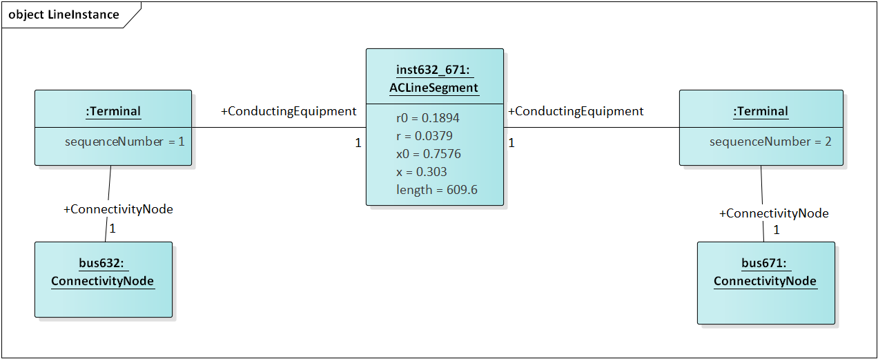
Figure 29: This is a balanced three-phase ACLineSegment between bus632 and bus671, 2000 feet or 609.6 m long. Sequence impedances are specified in ohms, as attributes on the ACLineSegment. This is a typical pattern for transmission lines, but not distribution lines.
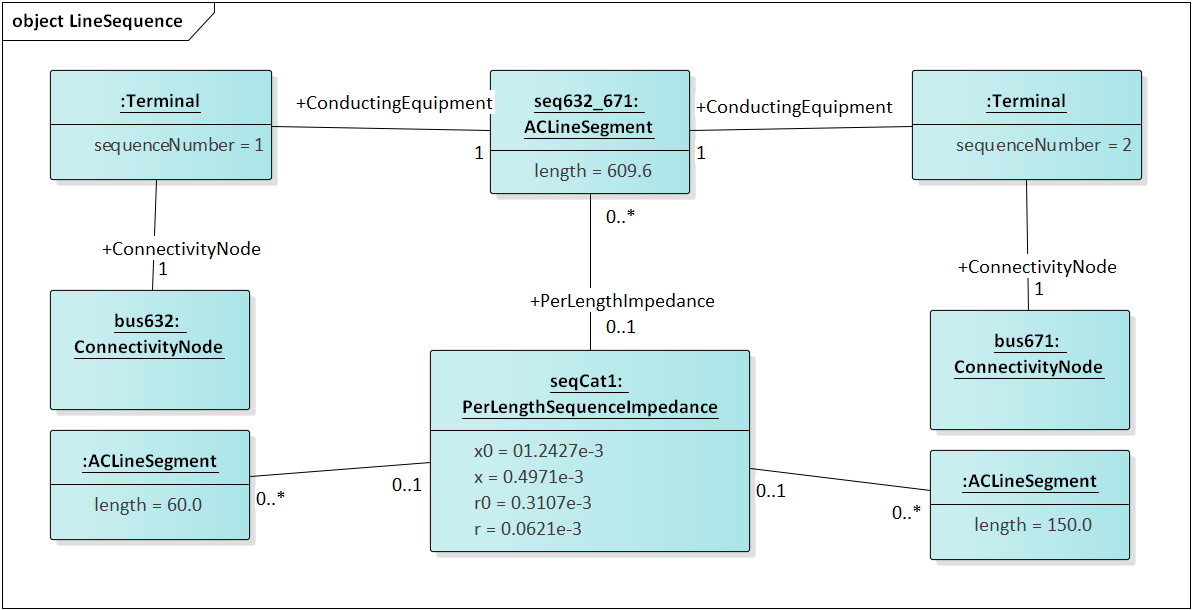
Figure 30: The impedances from Figure 24 were divided by 609.6 m, to obtain ohms per meter for seqCat1. Utilities often call this a “line code”, and other ACLineSegment instances can share the same PerLengthImpedance. A model imported into the CIM could have many line codes, not all of them used in that particular model. However, those line codes should be available for updates by reassigning PerLengthImpedance.
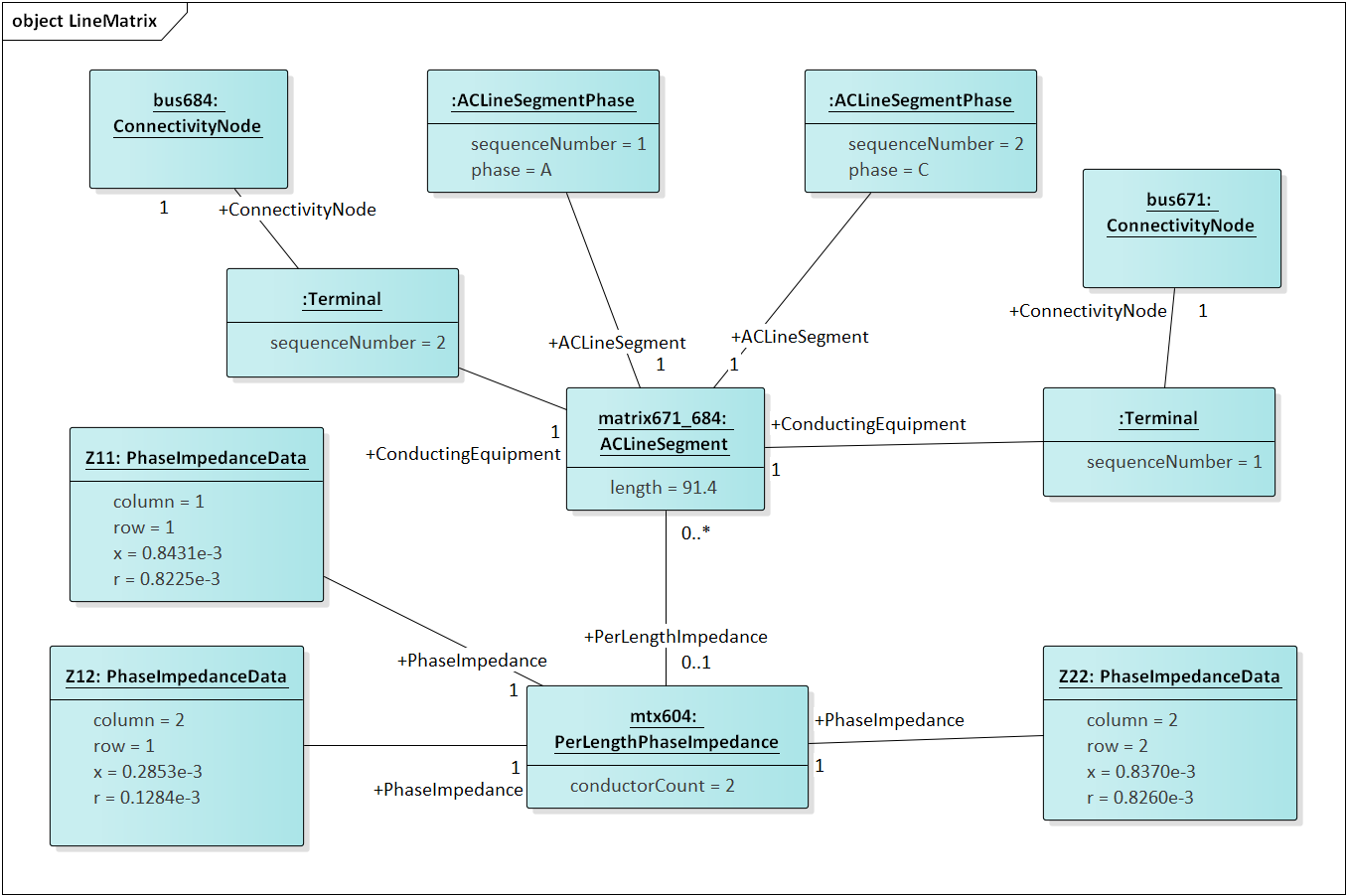
Figure 31: This is a two-phase line segment from bus671 to bus684 using a line code, which has been specified using a 2x2 symmetric matrix of phase impedances per meter, instead of sequence impedances per meter. This is more common for distribution than either Figure 29 or Figure 30. It’s distinguished from Figure 30 by the fact that PerLengthImpedance references an instance of PerLengthPhaseImpedance, not PerLengthSequenceImpedance. The conductorCount attribute tells us it’s a 2x2 matrix, which will have two unique diagonal elements and one distinct off-diagonal element. The elements are provided in three PhaseImpedanceData instances, which are named here for clarity as Z11, Z12 and Z22. However, only the row and column attributes are meaningful to identify the matrix element. In this example, Z11 and Z22 are slightly different. In order to swap phases A and C, we would swap the sequenceNumber values on the ACLineSegmentPhase instaces. As presented here, mtx604 can apply to phasing AB, BC or AC.
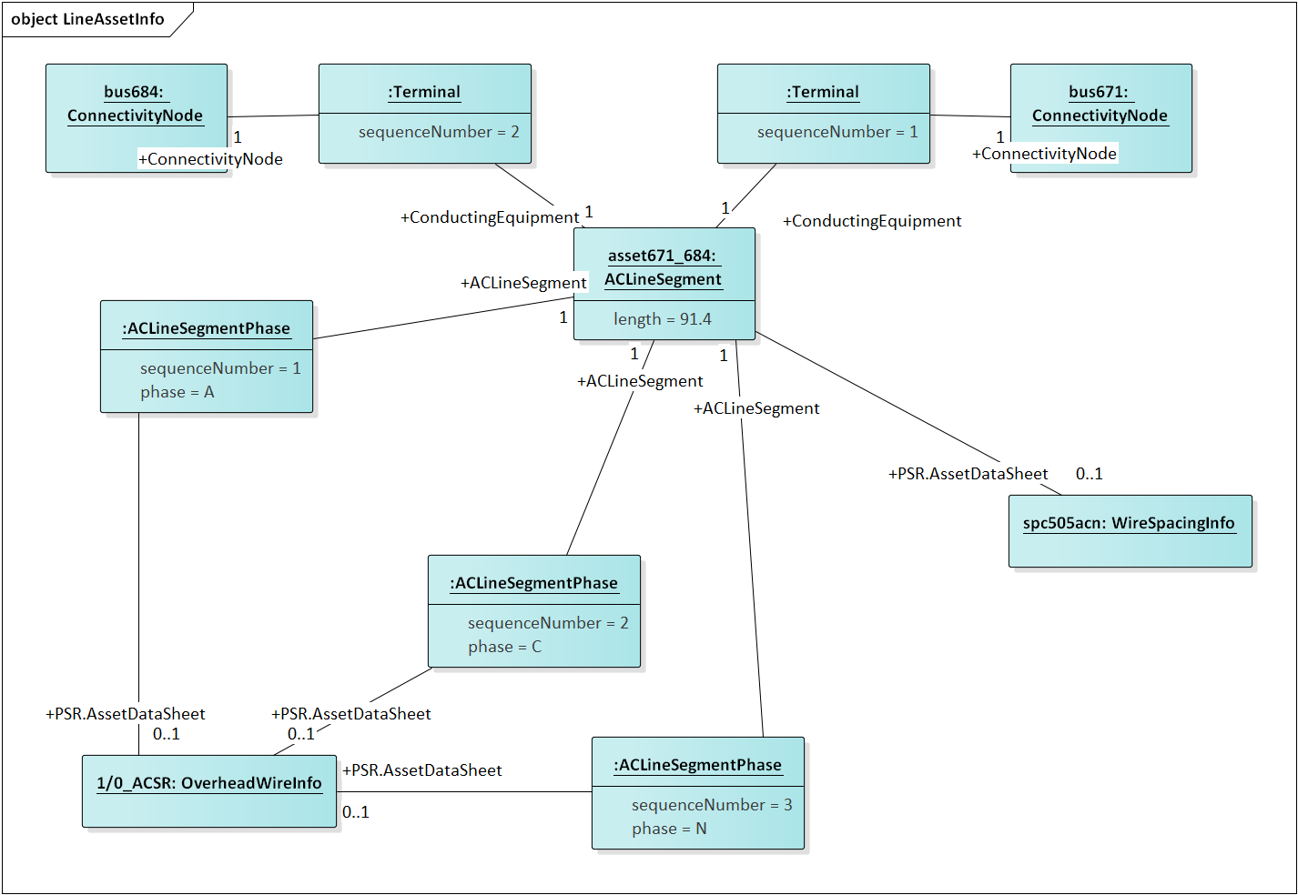
Figure 32: The two-phase ACLineSegment impedance defined by sharing wire and spacing data from a catalog. Each ACLineSegmentPhase links to an OverheadWireInfo instance via the AssetDataSheet association. If the neutral (N) is present, we have to specify its wire information for a correct impedance calculation. In this case, ACN all use the same wire type, but they can be different, especially for the neutral. Similarly, the WireSpacingInfo associates to the ACLineSegment itself via a AssetDataSheet assocation.
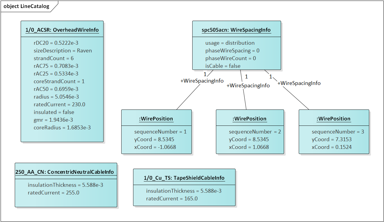
Figure 33: The upper five instances define catalog attributes for Figure 27. The WirePosition xCoord and yCoord units are meters, not feet, and they include sequenceNumber assignments to match ACLineSegmentPhase sequenceNumbers. The phaseWireSpacing and phaseWireCount attributes are for sub-conductor bundling on EHV and UHV transmission lines; bundling is not used on distribution. The number of WirePositions that reference spc505acn determine how many wires need to be assigned. Eliminating the neutral, this would produce a 2x2 phase impedance matrix. Although the pattern appears general enough to support multiple neutrals and transmission overbuild, the CIM doesn’t actually have the required phasing codes. When isCable is true, the WirePosition yCoord values would be negative for underground depth. To find overhead wires of a certain size or ampacity, we can put query conditions on the ratedCurrent attribute. To find underground conductors, we query the ConcentricNeutralCableInfo or TapeShieldCableInfo instead of OverheadWireInfo. All three inherit the ratedCurrent attribute from WireInfo. Cables don’t yet have a voltage rating in CIM AssetInfo, but you can use insulationThickness as a proxy for voltage rating in queries. Here, 5.588 mm corresponds to 220 mils, which is a common size for distribution.
Figure 34 illustrates the loads, which are called EnergyConsumer in CIM. The houses and appliances from GridLAB-D are not supported in CIM. Only ZIP loads can be represented. Further, any load schedules would have to be defined outside of CIM. Assume that the CIM loads are peak values.
Figure 35 illustrates the voltage regulator function. Note that GridLAB-D combines the regulator and transformer functions, while CIM separates them. Also, the CIM provides voltage and current transducer ratios for tap changer controls, but not for capacitor controls.
Figure 36 through Figure 38 illustrate how solved values can be attached to buses or other components.
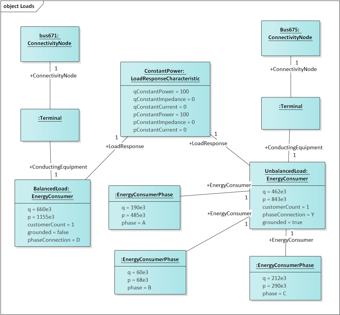
Figure 34: The three-phase load (aka EnergyConsumer) on bus671 is balanced and connected in delta. It has no ratedU attribute, so use the referenced BaseVoltage (Figure 19) if a voltage level is required. On the right, a three-phase wye-connected unbalanced load on bus675 is indicated by the presence of three EnergyConsumerPhase instances referencing UnbalancedLoad. For consistency in searches and visualization, UnbalancedLoad.p should be the sum of the three phase values, and likewise for UnbalancedLoad.q. In power flow solutions, the individual phase values would be used. Both loads share the same LoadResponse instance, which defines a constant power characteristic for both P and Q, because the percentages for constant impedance and constant current are all zero. The two other most commonly used LoadResponseCharacteristics have 100% constant current, and 100% constant impedance. Any combination can be used, and the units don’t have to be percent (i.e., use a summation to determine the denominator for normalization).
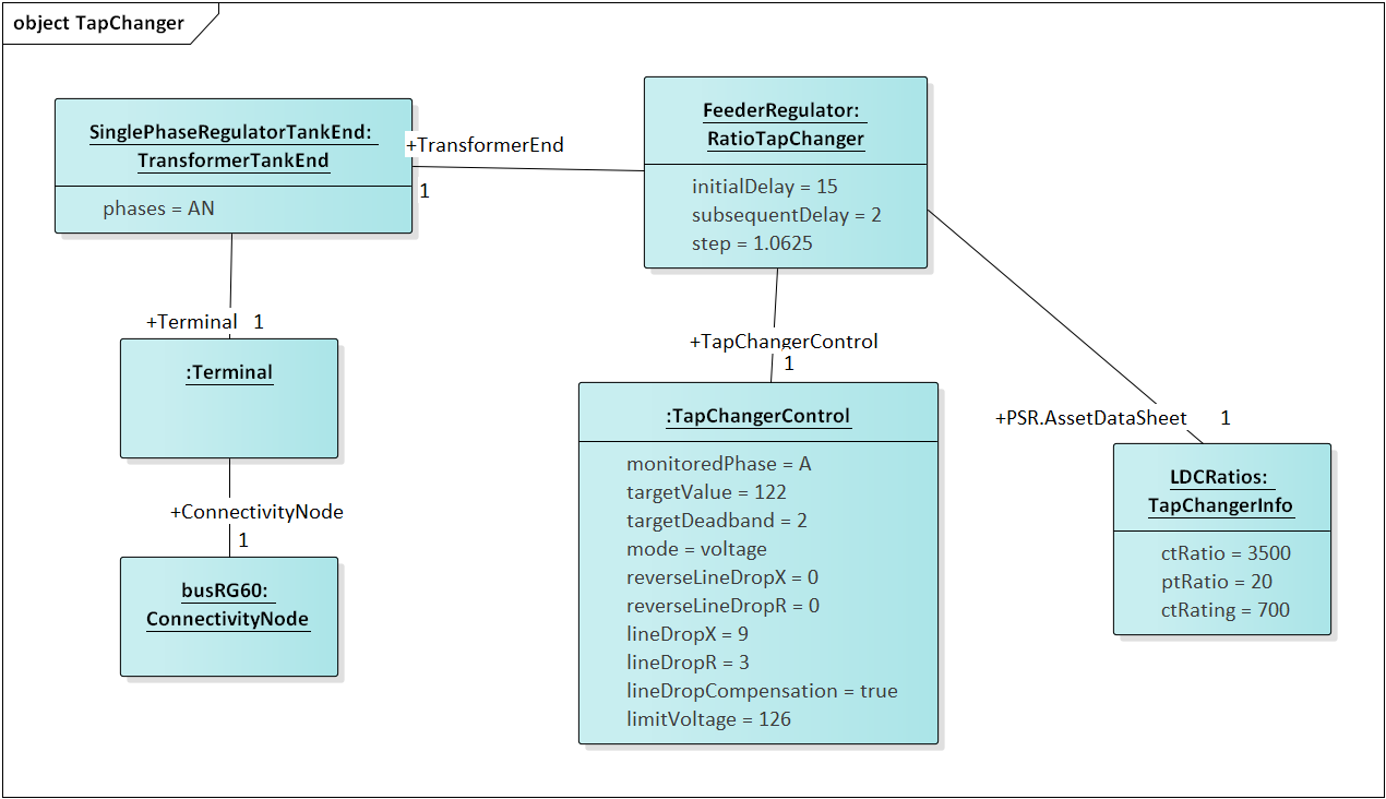
Figure 35: In CIM, the voltage regulator function is separated from the tap-changing transformer. The IEEE 13-bus system has a bank of three independent single-phase regulators at busRG60, and this example shows a RatioTapChanger attached to the regulator on phase A, represented by the TransformerTankEnd having phases=A or phases=AN. See Figure 25 for a more complete picture of TransformerTankEnds, or Figure 22 for a more complete picture of PowerTransformerEnds. Either one can be the TransformerEnd in this figure, but with a PowerTransformerEnd, all three phase taps would change in unison (i.e. they are “ganged”). Most regulator attributes of interest are found in RatioTapChanger or TapChangerControl instances. However, we need the AssetDataSheet mechanism to specify ctRatio, ptRatio and ctRating values. These are inherent to the equipment, whereas the attributes of RatioTapChanger and TapChangerControl are all settings per instance. For the IEEE 13-bus example, there would be separate RatioTapChanger and TapChangerControl instances for phases B and C.
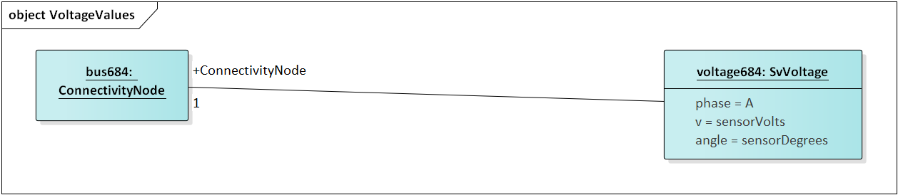
Figure 36: In this profile, a solved voltage value attaches to ConnectivityNode in GridAPPS-D. Positive sequence or phase A is implied, unless the phase attribute is specified.
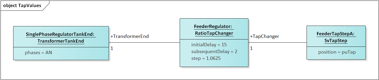
Figure 37: SvTapStep links to a TransformerEnd indirectly, through the RatioTapChanger. There is no phasing ambiguity because TransformerTankEnd has its phases attribute, while PowerTransformerEnd always includes ABC. Units for SvTapStep.position are per-unit.
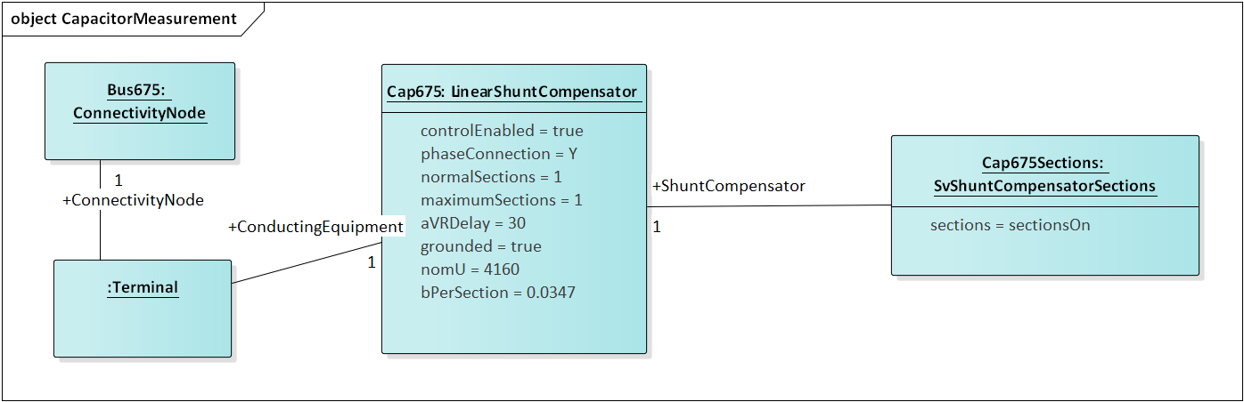
Figure 38: The on/off value for a capacitor bank attaches directly to LinearShuntCompensator. If the phase attribute is not specified, then this value applies to all phases.
Metering Relationship to Loads in the CIM
Figure 39 shows how emulated trouble calls will be connected to loads (EnergyConsumers) for test scenarios. The TroubleTicket is associated with Customer, CustomerAgreement and UsagePoint, which can then be associated to Equipment or any of its descendants. Figure 39 shows the linkage to EnergyConsumer or EnergySource, but it can also be linked to RegulatingCondEq (e.g., rotating machine and inverter-based DER). There are many attributes of Customer, CustomerAgreement and UsagePoint that are not yet used in GridAPPS-D, and not shown in Figure 40. These would be important for future metering and customer management applications. For now, the only TroubleTicket attributes to be used are dateTimeOfReport, resolvedDateTime and troubleKind. The PNNLTroubleCallKind was added because the existing troubleCode attribute is a non-standardized String. However, the comment attribute could be used for optional comments on each TroubleTicket.
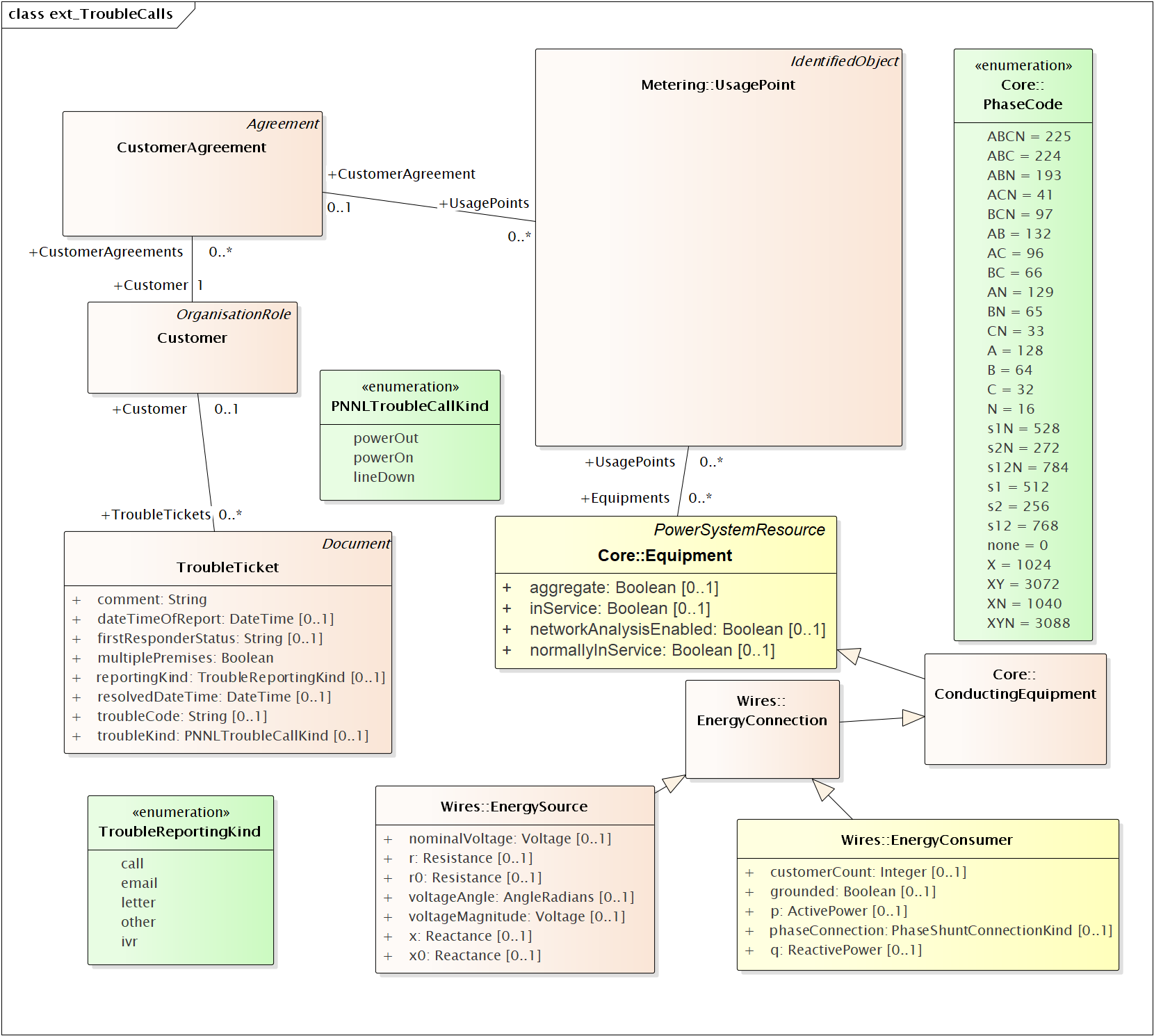
Figure 39: Trouble Calls route through Metering Usage Points to EnergyConsumers
CIM Enhancements for RC4
Possible CIM enhancements:
- Different on and off delay parameters for RegulatingControl (Figure 5)
- Current ratings for PerLengthImpedance (Figure 2). At present, some users rely on associated WireInfo, ignoring all attributes except currentRating.
- Transducers for RegulatingControl (Figure 5)
- Dielectric constant and soil resistivity (Figure 10)
- Clock angles for TransformerTankEnd (i.e. move phaseAngleClock from PowerTransformerEnd to TransformerEnd (Figure 6)
- Add the Fault.stopDateTime attribute
- Single-phase asynchronous and synchronous machines.
CIM Profile in CIMTool
CIMTool was used to develop and test the profile for RC1, because it:
- Generates SQL for the MySQL database definition
- Validates instance files against the profile
The CIMTool developer will not be able to support the tool in future, so we may use the new Schema Composer feature in Enterprise Architect when it’s ready for CIM profiling.
In order to view the profile, import the archived Eclipse project OSPRREYS_CIMTOOL.zip into CIMTool. Please see the CIM tutorial slides provided by Margaret Goodrich for user instructions.
Four instance files were validated against the profile in CIMTool. In order to generate them, we use a current version of OpenDSS with the Export CDPSMcombined command on four IEEE test feeders that come with OpenDSS:
- ~/src/opendss/Test/IEEE13_CDPSM.dss is the IEEE 13-bus test feeder with per-length phase impedance matrices and a delta tertiary added to the substation transformer. PV and storage were also added.
- ~/src/opendss/Test/IEEE13_Assets.dss is the IEEE 13-bus test feeder with catalog data for overhead lines, cables and transformers. Capacitor controls have also been added.
- ~/src/opendss/Distrib/IEEETestCases/8500-Node/Master.dss is the IEEE 8500-node test feeder with balanced secondary loads.
- ~/src/opendss/Distrib/IEEETestCases/8500-Node/Master-unbal.dss is the IEEE 8500-node test feeder with unbalanced secondary loads.
Either the 3rd or 4th feeder will be used for the volt-var application. The 1st and 2nd feeders are used to validate more parts of the CIM profile used in RC1. In all four cases, CIMTool reports only two kinds of validation error:
- Isolated connectivity node: CIMTool expects two or more Terminals per ConnectivityNode, but dead ended feeder segments will have only one on the last node. This is not really an error, at least for distribution systems.
- Minimum cardinality: For TapChangerControl instances, the inherited RegulatingControl.RegulatingCondEq association is not specified. This is not really an error, as the association is only needed for shunt capacitor controls. Figure 40 shows that RegulatingCondEq was not selected for TapChangerControl in the profile, so this may reflect a defect in the validation code. Efforts to circumvent it were not successful.
With these caveats, the profile and instances validate against each other, for feeder models that solve in OpenDSS.
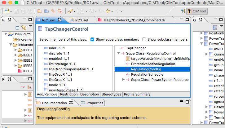
Figure 40: Editing a Profile in CIMTool
Legacy Data Definition Language (DDL) for MySQL
As shown at the top of Figure 40, CIMTool builds RC1.sql to create tables in a relational database, but the syntax doesn’t match that required for MySQL. The following manual edits were made:
Globally change CHAR VARYING(30) to varchar(50) with a blank space pre-pended before the varchar
Globally change “ to `
In foreign keys to enumerations, change the referenced attribute from mRID to name
In foreign keys to EquipmentContainer or ConnectivityNodeContainer, change the referenced table to Line
In foreign keys to ShuntCompensator, change the referenced table to LinearShuntCompensator
In foreign keys to TapChanger, change the referenced table to RatioTapChanger.
The CIM UML incorporates several polymorphic associations, which can’t be implemented directly in SQL. Base parent class tables were added for:
- AssetInfo, which can be referenced via the Parent attribute from ConcentricNeutralCableInfo, TapeShieldCableInfo, OverheadWireInfo, WireSpacingInfo, TapChangerInfo and TransformerTankInfo
- TransformerEnd, which can be referenced via the Parent attribute from PowerTransformerEnd and TransformerTankEnd
- PerLengthImpedance, which can be referenced via the Parent attribute from PerLengthSequenceImpedance and PerLengthPhaseImpedance
- Switch, which can be referenced via the SwtParent attribute from Breaker, Fuse, Sectionaliser, Recloser, Disconnector, Jumper and LoadBreakSwitch.
- ConductingEquipment, which can be referenced via the Parent attribute from ACLineSegment, EnergySource, EnergyConsumer, LinearShuntCompensator, PowerTransformer, and all of the Switch types.
The catalog data mechanism in Figure 8 required two new tables, one for polymorphic associations and another for many-to-many joins:
- PowerSystemResource, which can be referenced via the PSR attribute from ACLineSegment, ACLineSegmentPhase, RatioTapChanger and TransformerTank.
- AssetInfoJoin, which references AssetInfo and PowerSystemResource. This table actually supplants the Asset class in Figure 8.
The ShortCircuitTest in Figure 9 has a one-to-many association to TransformerEndEnfo, and we need to implement the many side by adding:
- GroundedEndJoin, which references TransformerEndInfo and ShortCircuitTest.
The ToTransformerEnd association in Figure 6 is one-to-many, so CIMTool did not export it to SQL. Rather than create a join table, a ToTransformerEnd attribute was added to TransformerMeshImpedance. This supports only one-to-one association, which is justified because the one-to-many case is very rare, and GridLAB-D cannot model transformers having the one-to-many association. This restriction may be removed in future versions having a semantic or graph database.
Except for the first two items, all of these adjustments arose from the absence of inheritance or polymorphism in SQL. These adjustments will make the updates, queries and views more complicated. However, they allow referential integrity to be enforced, which is one of the most important reasons to use SQL and relational databases. Other types of data store could be a more natural fit to the CIM UML, but they may not have the performance of a relational database.
In GitHub:
- RC1.sql is the manually adjusted SQL export from CIMTool
- LoadRC1.sql will re-create the GridAPPS-D database in MySQL, incorporate RC1.sql, and finally document the foreign keys. It should run without error.
| [1] | See http://cimug.ucaiug.org/default.aspx and the EPRI CIM Primer at: http://www.epri.com/abstracts/Pages/ProductAbstract.aspx?ProductId=000000003002006001 |
| [2] | Suggest “Corporate Edition” from http://www.sparxsystems.com/ for working with CIM UML. The free CIMTool is still available at http://wiki.cimtool.org/index.h tml, but support is being phased out. |
| [3] | OSPRREYS is an older name for GridAPPS-D |
| [4] | https://github.com/GRIDAPPSD/Powergrid-Models/CIM |
Platform UML Diagrams
UML from the Functional Specification
This section presents a selection of GridAPPS-D domain (class) diagrams to supplement the OSPRREYS Functional Specification document. The purpose is to enhance understanding of the functional specification, by providing graphical walkthroughs of some important use cases. The reader should be familiar with definitions in the functional specification, and with Universal Modeling Language (UML) diagrams.
GridAPPS-D is organized as a suite of internal function managers, twelve of them composing the Platform Manager as shown in Figure 1. All GridAPPS-D functions and interactions are mediated by one (or more) of these function managers. When running, the GridAPPS-D 413 Platform Manager will be composed of one (and only one) of each internal manager numbered 401 – 412. These internal managers work together to accomplish various GridAPPS-D functions.
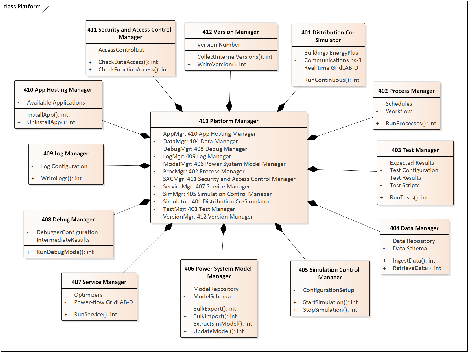
Figure 1: Composition of the GridAPPS-D Platform Manager
Within each class block, some top-level attributes are listed with (-) signs in the middle division, and some top-level methods are listed with (+) signs in the lower division. For example, we already know that 401 Distribution Co-Simulator will need component simulators (i.e. attributes) for buildings (open-source EnergyPlus), communications (open-source ns-3), and the electric power distribution grid (open-source GridLAB-D running in a real-time mode). It will also need at least one method that runs the suite of simulators in a mode emulating continuous real-time operation. Taking another example, 407 Service Manager also contains an attribute for GridLAB-D to provide power flow calculations, but run as a service to applications.
As the design evolves, classes in Figure 1 will acquire many more attributes and methods. The attributes themselves may reference complicated classes and data structures. Therefore, the UML model will expand each class into layer and sub-layer diagrams to more clearly show these evolving details. We can still use the top-level diagrams to make sure that the major components are in place for the important use cases.
Figure 2 illustrates the case of a user executing an application, in the role of EF7 from the functional specification. We initially focused on volt-var optimization (VVO), and then added a more complicated demand response (DR) application that fits the same basic pattern. As a prerequisite, some entity has provided both applications to GridAPPS-D for registration and hosting, in a process detailed later. For now, we assume the application(s) have been installed and will focus first on running VVO.
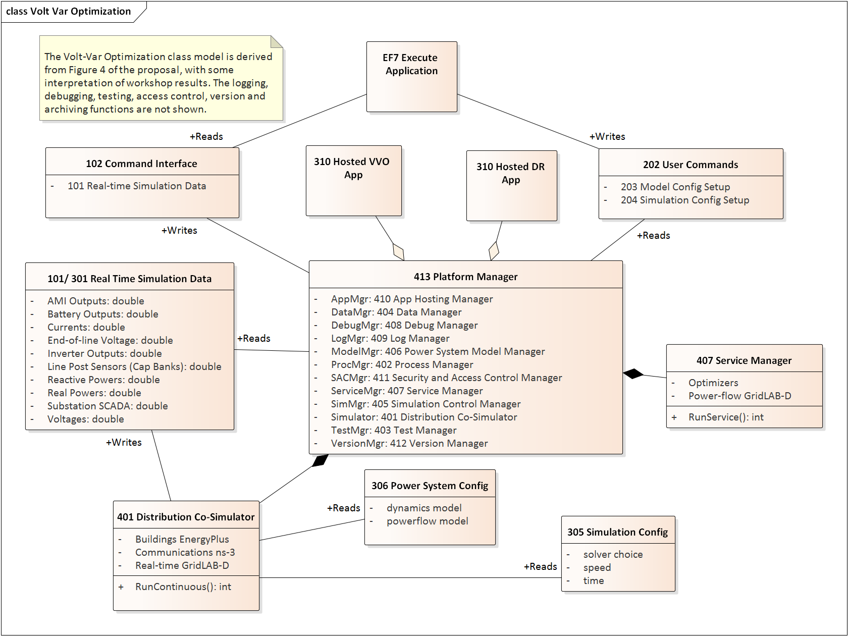
Figure 2: Executing an application
All user interaction with GridAPPS-D occurs through a command interface, numbered 202 when the user writes commands to GridAPPS-D, and numbered 102 when the user gets data from GridAPPS-D. To run VVO, the user will issue 203 Model Configuration Setup and 204 Simulation Configuration Setup to GridAPPS-D, which then delegates the commands to various internal function managers (see Figure 1). The 203 Setup will probably extract the feeder model of interest, set load and weather data, etc. The 204 Setup will probably tell 401 to run GridLAB-D for a certain time period, but not to run ns-3 or EnergyPlus. The exact composition of 203 and 204 Setups will be determined later in the design process. In a process described later, internal functions 405 (Simulation Control Manager) and 406 (Power System Model Manager) will transform 201, 203 and 204 into 305 and 306, which 401 can then read and run from directly.
When it runs, 401 will generate streams of data that mimic real-time operation of the system, and these streams pass to the other parts of GridAPPS-D as 301 Real-time Simulation Data. Some of the data streams may also output to the user as 101 Real-time Simulation Data. The 310 VVO Application can act on this data to make decisions (e.g. switch capacitor banks, change regulator taps, change solar inverter settings). In this process, 310 VVO could invoke power flow calculations in GridLAB-D via 407 Service Manager, but this is different from the way 401 Co-Simulator runs. The application may use 407 services to explore alternatives or run contingency analysis, which could change the power system model, but the 401 real-time simulations always take priority and always use the “real” model.
When we considered adding the second and more complicated application, 310 DR, the structure of Figure 2 didn’t change very much. The open-headed diamond symbols indicate that GridAPPS-D can host several applications, which is UML aggregation. These applications may interact via the GridAPPS-D command interface, if the applications and their command sets have been designed for it. For example, the DR application may use VVO to check and mitigate voltage limits.
A DR application is more likely than VVO to need EnergyPlus and ns-3 in the co-simulation. In response, we added those attributes to 401, and will add supporting attributes to 201, 203 and 204 as the design evolves. It should also be recognized that more sophisticated VVO applications might incorporate communications (ns-3) if available.
Figure 3 depicts the process of managing power system models, including the schema and repository within 201 Distribution System Model. Because it’s based on standards (e.g. IEC 61968) and open-source tools (e.g. MySQL), the model can be created and maintained from outside GridAPPS-D, directly by EF 21, the Model Manager. This is shown at the top of Figure 3. This process is out of GridAPPS-D scope but within project scope, and it can leverage existing tools like Cimphony, Cimdesk, EA, etc.
For use by and within GridAPPS-D, all model configuration commands will pass from EF21 through the command interface to function 406, the Power System Model Manager. This function reads the base power system model data from 201, and configures it into a three-phase load flow model for solution in 106/306. The Distribution Co-Simulator uses 306, but the user might want 106 for off-line use. Working with 404 Data Manager, the 406 Power System Model Manager may also write additional data (i.e. not used in the load flow calculation) to 104/304. In this case, the 102 Model Output function will collect that data from both 104 and 106 for reporting to the user, EF7, via the command interface. Note that the base data, in 201, is not modified through this process. Instead, the base data is treated as input to GridAPPS-D.
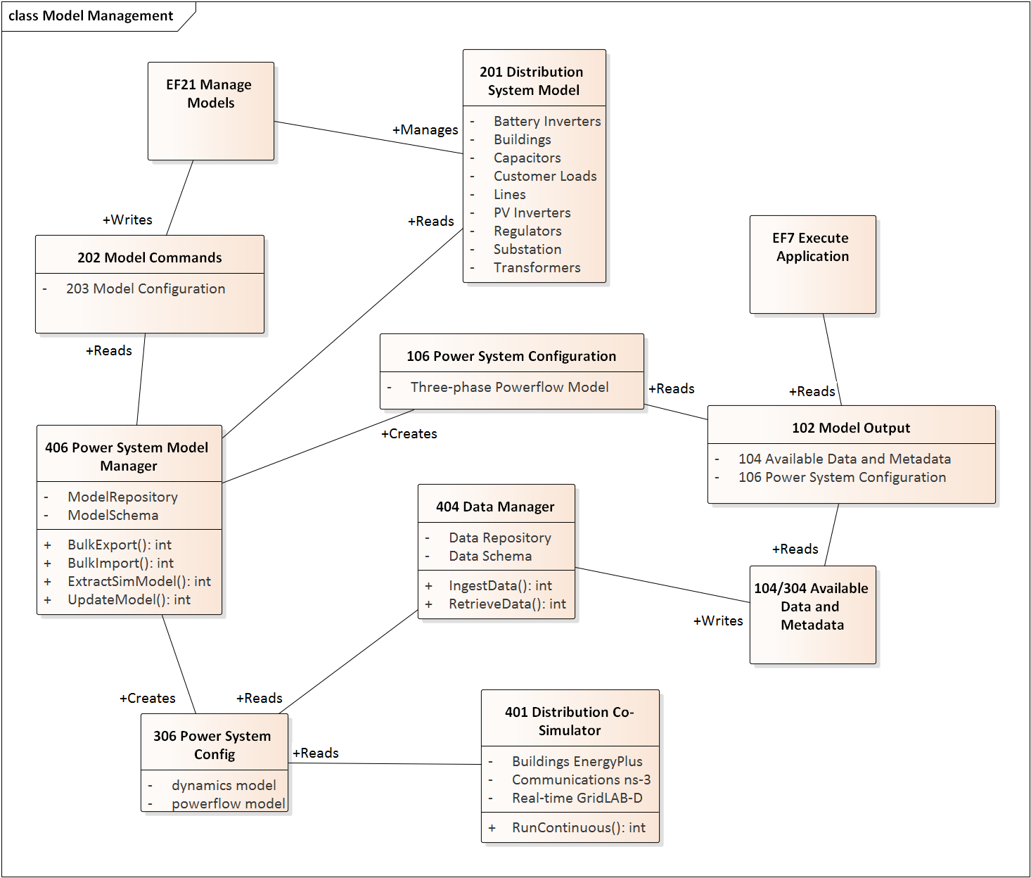
Figure 3: Internal model management
Figure 4 shows the internal Platform Manager flow when running application tests. Compared to the case of normal usage in Figure 2, this example shows additional control and output for testing. The test commands include 203 and 204, as in Figure 2, but they also include:
- 205 Test Scripts, for the sequence of steps to perform
- 206 Test Configuration Setup, including initial conditions, etc.
- 207 Expected Results, for comparison to the actual output
- 210 Application Metadata, for information to run and instrument the application
The 403 Test Manager orchestrates the steps to run the application and collect results. As part of 103 Test Results, it will compare the real-time data (101/301) to the expected results in 207. If the testing user, EF8, requested logging, then the 409 Log Manager will create 109/309 System Logs for collection by 403 Test Manager. Logging is optional, and should have been requested as part of the 206 Test Config Setup or 204 Model Config Setup (this is not spelled out in the functional specification).
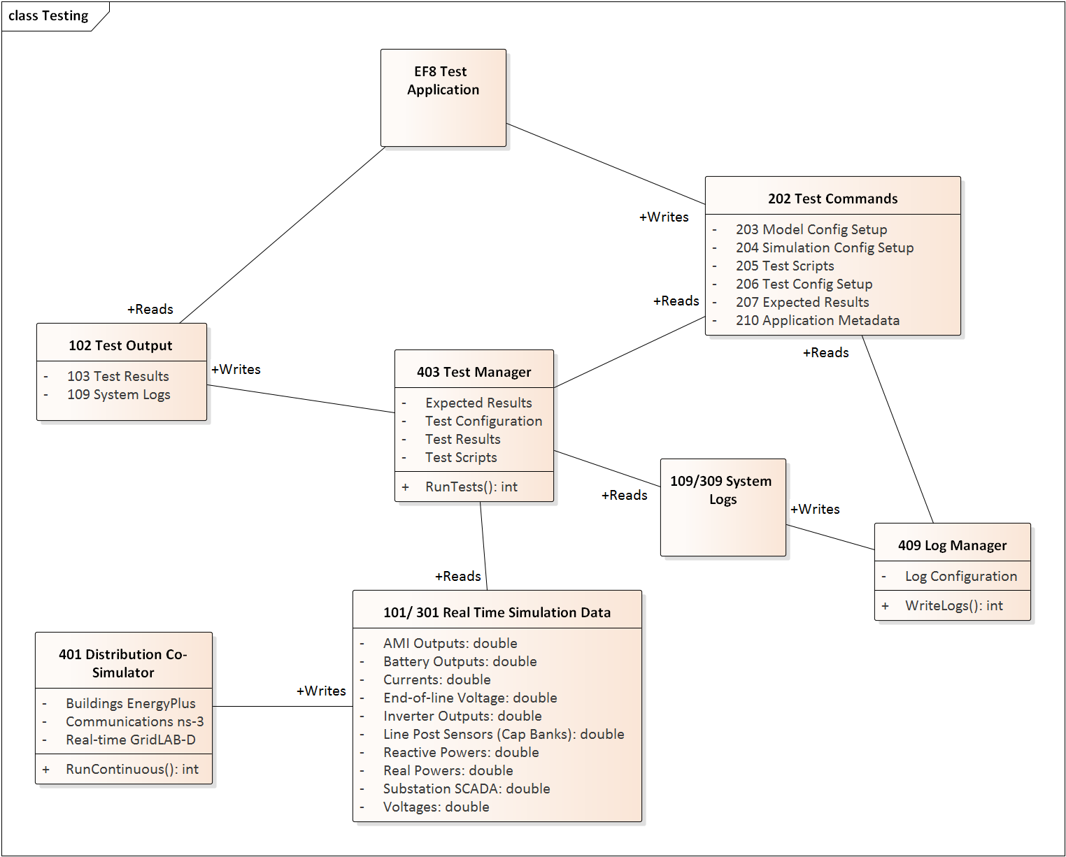
Figure 4: Testing an application or the platform
Figure 5 shows some of the internal 413 Platform Manager detail when a user, EF7, runs an application in debugging mode. Compared to Figure 2, there is much more internal output. The 212 Debug Configuration will include such things as breakpoints, watch variables, and logging requests. When run in debug mode, the 408 Debug Manager will collect the internal inputs and intermediate results from a variety of GridAPPS-D modules, including the simulator, services in use, model data, and access violations. The 404 Data Manager mediates most of this data collection (and with a change to the specification it could also mediate 101/301). The 408 Debug Manager combines this into 108 Intermediate Results, with 109 System Logs, for output to the user via the command interface. Depending on the implementation of GridAPPS-D, interactive debugging may also be supported, but is not shown in Figure 5.
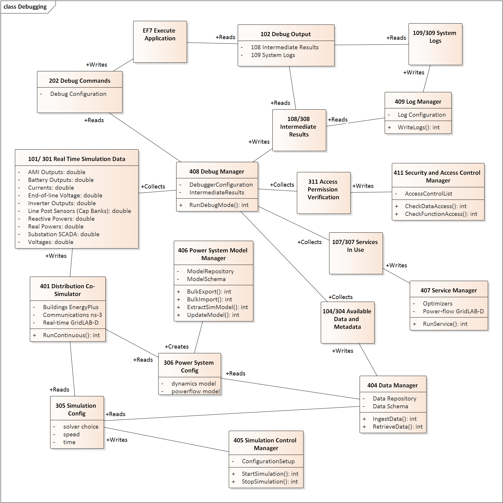
Figure 5: Debugging an application
Figure 6 shows the process of registering or updating an application to use with GridAPPS-D. The developer, in the role of EF13, must provide the application itself (211) along with the application data schema (208) and metadata (210). The data schema includes input and output parameters. The metadata includes a user-friendly name, description, calling parameters, command syntax, API functions used, etc. Using this information, 410 Application Hosting Manager will install and register the application, and its data, with 407 Service Manager and 404 Data Manager. After completing these steps, 412 Version Manager will output the current version information via the command interface; the current version includes information about which applications are installed along with the application versions.
In order to perform application management, EF13 also needs to provide user credentials to be checked against the 209 Access Control List. If these credentials are valid, the 411 SAC Manager will create 311 Access Permission Verification for all of the internal Platform Manager components. In Figure 6, the 410 Application Hosting Manager can pass 311 to 404, 407 and 412 as needed. Although not shown earlier, SAC is actually incorporated into all GridAPPS-D processes this way.
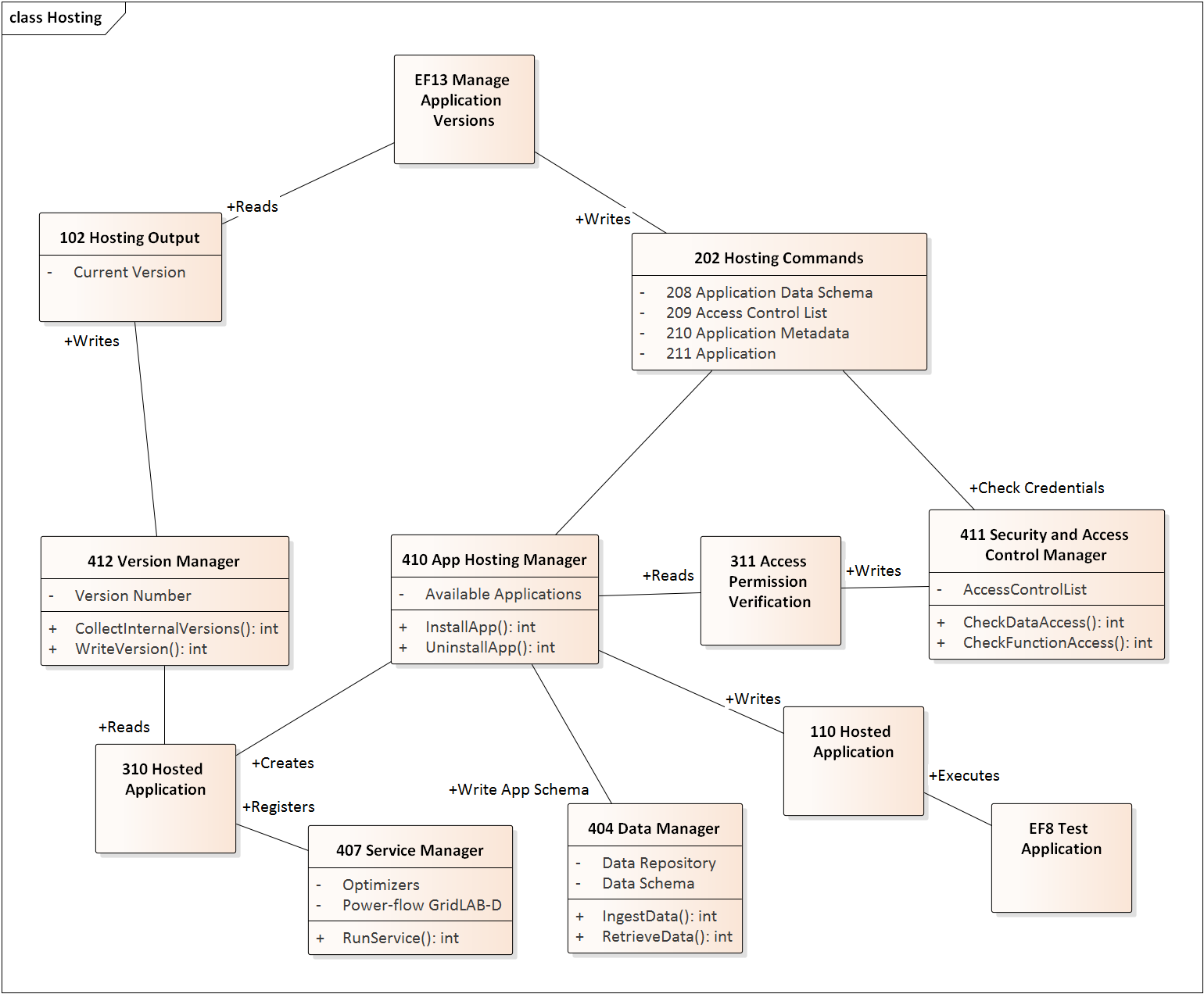
Figure 6: Hosting an application
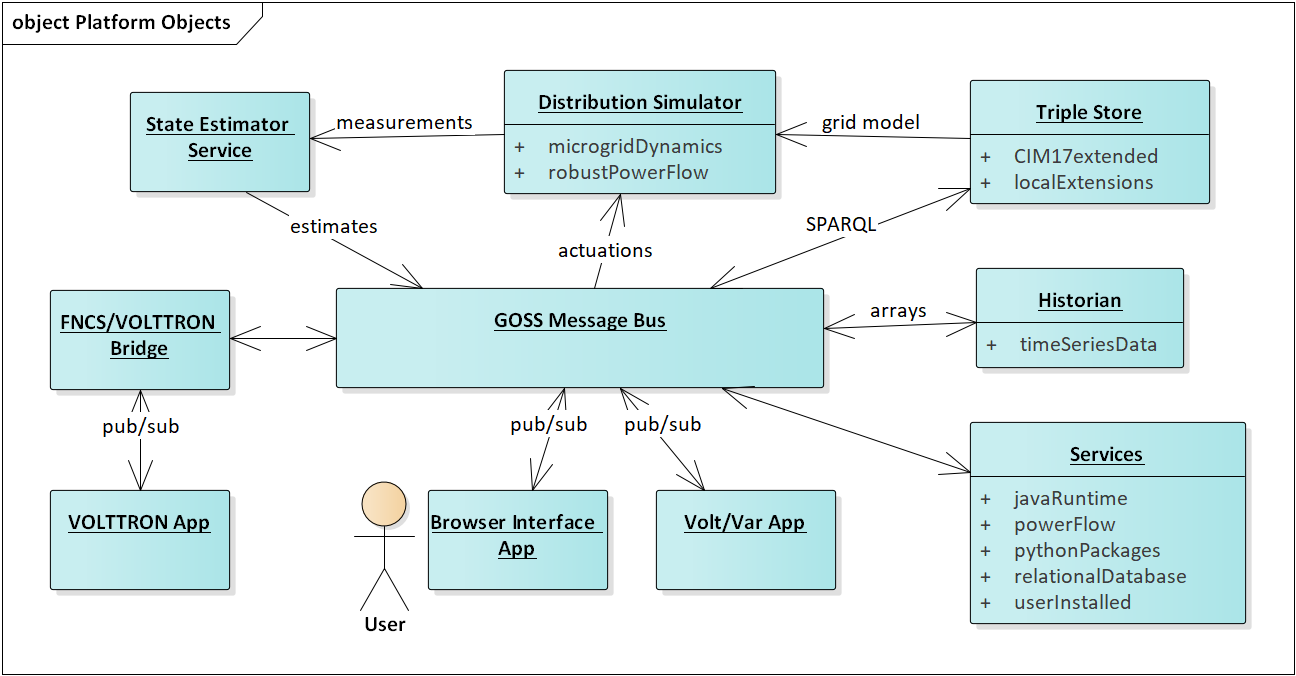
Figure 7: Platform Objects
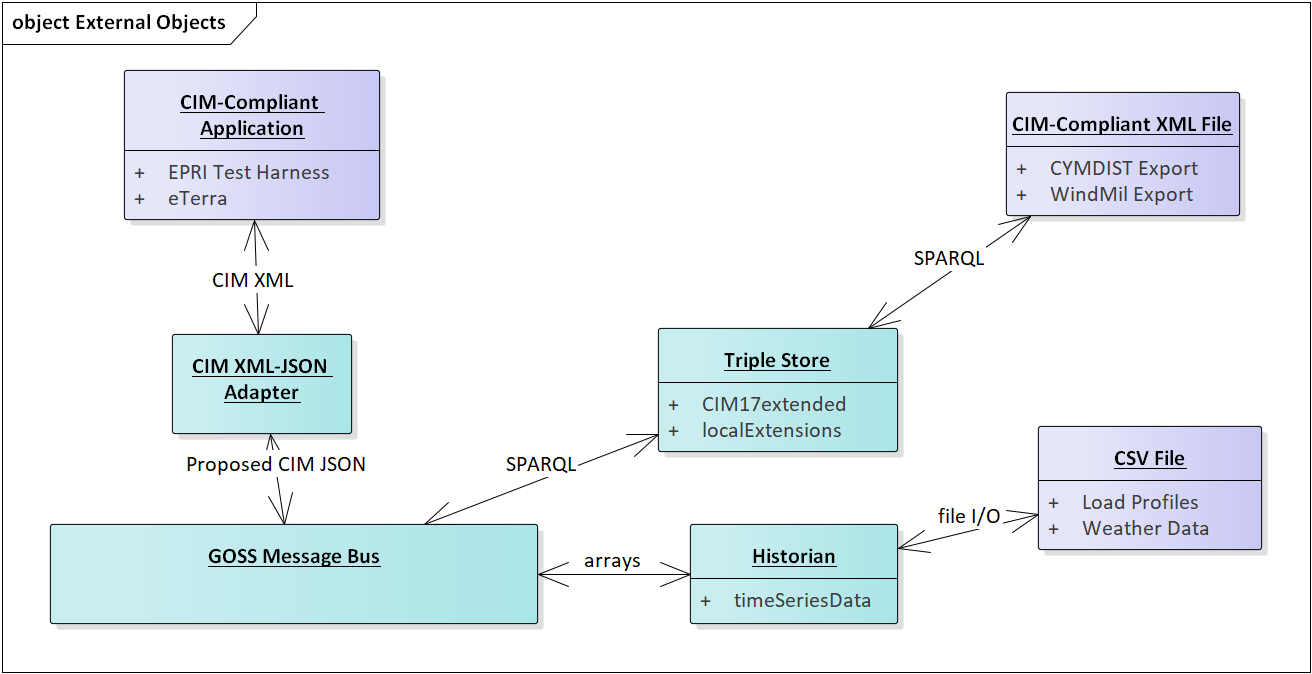
Figure 8: External Objects
UML for Release Cycle 4
Our objective is to demonstrate useful functionality, which is standards-compliant, by the end of March 2017. A simple heuristic VVO application will be running in GridAPPS-D. In terms of the Functional Requirements, we will be implementing:
- 102/202 Command Interface
- 301 Real-time Simulation Data
- 310 Hosted Application, but short-cutting the registration process
- 401 Distribution Co-Simulator (partial)
- 402 Process Manager (partial)
- 404 Data Manager (partial)
- 405 Simulation Manager (partial)
- 406 Power System Model Manager (partial)
- 413 Platform Manager (encapsulating 401 and 403-406)
This represents five out of twelve Internal Functions from the Functional Requirements, in partial form. The deadline leaves four months for detailed design and implementation, plus two months for documentation and testing. Therefore, we have chosen a minimal set of functions that can show end-to-end use of GridAPPS-D at the first milestone.
In developing the work breakdown structure (WBS), we noted that real-time simulation data is published with no time lags or errors in Release 1. However, data flow in a real DMS is affected by sensor and communication system performance, and also by the action of other subsystems. In Release 2, this might be addressed through some combination of:
- Communication and sensor models in the Distribution Co-Simulator
- Adding MDM and SCADA service attributes to the 407 Service Manager
- Filters on 301 Real-time Simulation Data
These decisions, and many others affecting Release 2 and Release 3, can be deferred until we gain experience developing Release 1.
Figure 1 shows the software components planned for Release 1. Most of these correspond to internal functions from the Functional Requirements, with some relatively minor re-factoring. The Power System Model Manager functionality has been split. The data store management and the creation of a complete GridLAB-D model appear at the bottom. Once the simulator is running, incremental changes are posted to the messaging bus.
Most of the “pink” components in Figure 1 are assigned to one task, except:
- The 310 VVO is a sub-task of the Command Interface, due to the close coupling of those efforts. The team on this task needs both power system and software skills.
- A separate task has been added for some project-level items.
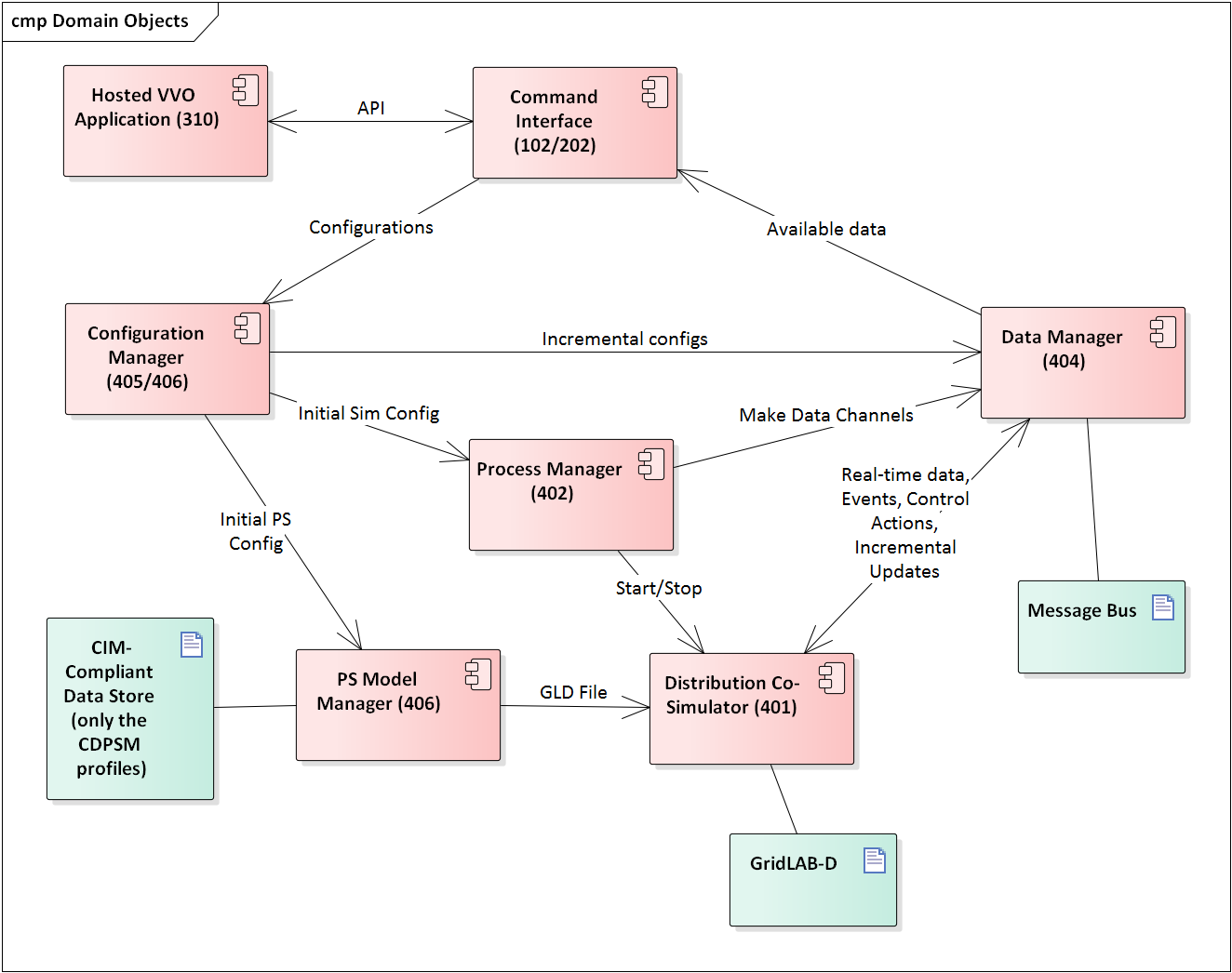
Figure 1: Component Diagram for GridAPPS-D Release 1
Initial Work Breakdown for Release Cycle 1
The Release 1 work breaks down into seven tasks, listed below. Three critical items must be completed first; these are highlighted in red. There are other inter-task dependencies that have not yet been called out. We plan to sequence the work over eight two-week “sprints” within the four months allocated for detailed design and development, using an agile process (Kanban).
- Project-level Elements
- Identify a power system model (note: IEEE-13 is already in CIM/CDPSM)
- Design data store schema
- Manually ingest power system models
- Command Interface
- Design APIs
- For all configurations in Task 4
- For power system control actions (e.g. open/close switch)
- Select one language binding (e.g. Python, Java, C++, MATLAB) and implement
- Develop a heuristic volt-var application (VVO) in the bound language
- Integrate VVO into GridAPPS-D
- Design APIs
- Messaging and Data Manager
- Select a messaging framework (eg. ZeroMQ)
- Create communication APIs
- Receives real-time data from simulator
- Receives power system control actions
- Handle communication between GridAPPS-D managers
- Log messages to file
- Configuration Manager (both Power System Config & Simulation Config)
- Receive configurations from command interface over message bus
- Translate configurations to native GridLAB-D
- Translate and publish incremental update messages
- Send configurations to Process Manager for simulation start
- Process Manager
- Receives configurations from the Configuration Manager
- Send configuration to the Distribution Co-Simulator
- Start Co-Simulation Process
- Create simulation data channels and inform application
- Stop simulation process
- Distribution Co-Simulator (wraps GridLAB-D)
- Accepts configurations from Process Manager
- Start simulation
- Produce and publish data in real time
- Accept changes in real time (e.g. capacitor switching) via message bus
- Power System Model Manager
- Access the power system model in data store
- Create native GridLAB-D file for initial loading into the simulator
CIM Validation
This section presents an overview of CIM Validation techniques that will be expanded upon in the future. The purpose of CIM validation is to assess the level of compliance GRIDAPPS-D is using in its use of CIM version 100.
Introduction
In electrical power distribution and transmission the Common Information Model (CIM) is a technology agnostic standard developed by the International Electrotechnical Commission (IEC). CIM provides the blueprints for application software like GridAPPS-D to represent data structures, message payloads, and information exchanges between applications.
To represent the model, CIM is written using the Unified Modeling Language (UML) using Sparx Enterprise Architect. The model is stored in a project file (*.eap extension file).
UML Profiles are domain or technology specific representations of the original model. UML profiles are generated in a variety of ways: including: by hand, using a tool such as CIMContextor/CIMTool.
Extending CIM
CIM is built on universally understood power grid concepts which means that the UML should be generally applicable, When the needs go beyond the general purpose solution it is possible to extend CIM for application specific purposes. When extending CIM to be compliant, the extentions comply with the rules and organization of the existing model. Otherwise an uncompliant application risks losing the advantage of using the standard, particularly for information exchanges.
Techniques for extending the CIM will not be discussed here, however the IEC TC 57 61970 part 301 document provides excellent guidance on best practices when extending the CIM. The 61970 part 600 series developed for use by ENTSO-E provides an excellent end-to-end series of extension use cases for the European power grid.
Validation Techniques
Well-Formed UML Compliance
In the IEC TC 57 13, 14, and 16 Working Groups the CIM Model Managers are relied upon for any updates to the UML. Before a release occurs the JCleanCim tool (http://tanjakostic.org/jcleancim/index.html) is used to validate UML package, class, and associations against agreed upon rules for well-formed UML. The JCleanCim tool generates a log report citing any non-compliance items along with other products. It is basically like a software debug tool for CIM UML. For extensions the JCimClean tool can be used to review GridAPPS-D extensions and flag any problematic areas. In addition the JCimClean tool original log report for CIM100 can be compared against the GridAPPS-D CIMv100.
Well-Formed Profile
Two external tools have been developed to create CIM profiles based on the UML. Both CIMTool and CIMContextor can create Resource Description Framework Schema (RDFS) profiles from CIM to validate how CIMv100 classes and associations are transposed into message payload objects. In addition, CIMTool does have a means to validate example payloads against payloads to flag any formatting or structural errors.
Final Thoughts
This section is expected to evolve in the spring/summer of 2019 with the advancement of CIM Model Manager tools that were previously only accessible to the model managers or based on advancements of validation techniques in the profile development communities.